Survival Analysis for MIP Solving Time

Survival Analysis for MIP Solver Running Time

Inspired by the recent activity in open-source MIP solvers (HiGHS is becoming stable after the 1.0 release and many users submitting bug reports, SCIP has become open-source software), I wanted to revisit some folklore about running times.

When solving difficult problems, in particular, when running computational experiments, we have to choose a timelimit to tell the solver when to give up solving the problem (that is finding a solution and proving its optimality). If the timelimit is chosen too small, many instances will not be solved within it and therefore we can not compare the running time between different solvers or settings. But if we set the timelimit to long, we might waste computational resources while waiting for a result that never comes.

I remember the rule of thumb:

If the problem is not solved within an hours, it will also not be solved after four hours (or later).

Let's see if we can use some data and survival analysis to confirm this rule.

In [1]:
from lifelines import KaplanMeierFitter
import matplotlib.pyplot as plt
import pandas as pd
In [2]:
def make_ax():
    fig = plt.figure(figsize=(12, 9))
    ax = fig.subplots()
    return ax

Data Prep

We use running time data from the Mittelmann benchmarks on the MIPLIB set of benchmark instances, a set of representative difficult MIP instances.

From the solver comparison, we only look at the open-source solvers still in active development: HiGHS and SCIP. The timelimit was set as 2 hours (7200 seconds), which we use as our window of observation. The tables contain either the time to optimality (solved instance) or some exceptional status (either timout or an error). We interpret all exceptions as right-censored data.

In [3]:
# Read in MIPLIP results (subset of solvers, converted to CSV)
times = pd.read_csv("../files/miplib_20221113_8threads.csv")
times.head()
Out[3]:
Instance HiGHS SCIP
0 30n20b8 537 69
1 50v-10 5508 timeout
2 academictimetablesmall timeout timeout
3 air05 22 24
4 app1-1 23 3
In [4]:
# Bring table in long form, not separate columns per solver
times = pd.melt(times, id_vars="Instance", var_name="Solver", value_name="Runtime")
times.set_index(["Solver", "Instance"], inplace=True)
In [5]:
# Replace exceptional status with time limit
for status in ["abort", "mismatch", "timeout"]:
    times.replace(status, 7200, inplace=True)

# Convert all values to numbers
times["Runtime"] = times["Runtime"].astype(float)
In [6]:
# Identify the instances that have been solved properly within the time limit.
# The others are right-censored, that is, we don't know how long it would have taken to solve them,
# including cases with an error status.
times["Finished"] = 1 * (times["Runtime"] < 7200)
times.head()
Out[6]:
Runtime Finished
Solver Instance
HiGHS 30n20b8 537.0 1
50v-10 5508.0 1
academictimetablesmall 7200.0 0
air05 22.0 1
app1-1 23.0 1

Kaplan-Meier Estimate

We apply the Kaplan-Meier estimate to draw survival curves for each solver.

These show the probability that an instance has survived for some time (ie, has not yet been solved to optimality), together with a 95% confidence interval.

Note that the curves (one for each solver) start at 100% for time 0 and decrease monotonically. The curves stop at 7200s (the time limit set) but have not reached 0%, because of some instances that have not been solved.

We can see a steep decline in the first few minutes, while the curves flattens to a long tail, as predicted by our rule of thumb.

In [7]:
def kaplan_meier(solver, ax=None):
    kmf = KaplanMeierFitter()
    kmf.fit(
        times.loc[solver]["Runtime"],
        event_observed=times.loc[solver]["Finished"],
        label=solver,
    )
    return kmf.plot_survival_function(ax=ax)
In [8]:
ax = make_ax()
for s in ["HiGHS", "SCIP"]:
    kaplan_meier(s, ax)

Conditional Survival

We can also look at conditional survival, considering only that part of the curves beyond the first hour. That is, we reframe our questions from

What is the probability that an instance has survived (not been solved) after some time?

to

What is the probabilty that an instance is solved after some time of additional waiting, knowing that it wasn't solver after the first hour?

To that end, we merge the data from both solvers and make some adjustments to the resulting survival curve.

In [9]:
kmf = KaplanMeierFitter()
kmf.fit(
    times["Runtime"],
    event_observed=times["Finished"],
    label="Open Source Solvers"
)
ax = make_ax()
kmf.plot_survival_function(ax=ax);
In [10]:
# Only keep right tail of curve, going beyond 1h
survival = kmf.survival_function_["Open Source Solvers"]
tail = survival[3600:]
tail.index = tail.index - 3600.0
In [11]:
# Rescale probability to start at 100% (conditional on surviving 1h),
# and negate the probability (solving it within time).
cond_tail = 1.0 - tail / tail.iloc[0]
In [12]:
# Visualize probability of solving it after waiting for additional time, after 1h.
ax = make_ax()
cond_tail.plot(ax=ax, drawstyle="steps-pre");

The above chart shows the probability than instance is solved after some time (beyond 1h), given that it wasn't solved already. It tells us that an additional hour of computation would only solve about 10% of the remaining instances.
The Food Triangle Quantified

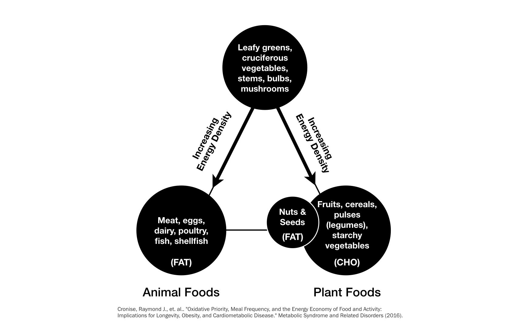
In a recent cookbook, the Healthspan Solution, the authors propose a new way to categorize food: the food triangle.

First of all, only whole food ingredients are considered. Then, rather than grouping foods into one of the macronutrients (fat, protein and carbohydrates), they are sorted by energy density on the one hand (top / down), and by source (animal on the left, plants on the right) on the other:

Food Triangle

The recommendation is to eat on the "right side", in particular near the top, in order to get sufficient micronutrients while keeping energy intake in check.

On the other hand, many traditional recipes choose foods from both sides near the bottom, yielding the highest energy density while promoting fat storage due to oxidative priority.

I like this scheme, but I wondered whether most foods could really be assigned one of these sides easily. So this post is about visualizing foods by their energy density and relative source of energy (fat vs carbohydrates).

In [1]:
# Activate custom environment ad load packages
using Pkg
Pkg.activate("../../environments/food-triangle/");

using CSV
using DataFrames
using VegaLite
 Activating environment at `~/src/rschwarz.github.io/environments/food-triangle/Project.toml`
In [2]:
# Load nutrition data
foods = DataFrame(CSV.File("../files/foods.csv"))
@show size(foods)
first(foods, 3)
size(foods) = (142, 7)
Out[2]:

3 rows × 7 columns

Source Category Food Energy Protein Fat Carbohydrates
String String String Float64 Float64 Float64 Float64
1 Plant Grain Oats 272.0 2.4 1.6 10.1
2 Plant Grain Barley 388.0 2.9 0.9 18.0
3 Plant Grain Buckwheat 304.0 2.5 0.6 14.1

Energy

Our nutrition data lists 142 different foods from different categories with energy (in kJ per 100g) as well as relative weight of the macronutrients.

Since fat has a much higher energy density, we will replace the weight values by the energy contribution per macronutrient.

In [3]:
foods.Fat = 37.0 .* foods.Fat
foods.Carbohydrates = 16.0 .* foods.Carbohydrates
foods.Protein = 17.0 .* foods.Protein
first(foods, 3)
Out[3]:

3 rows × 7 columns

Source Category Food Energy Protein Fat Carbohydrates
String String String Float64 Float64 Float64 Float64
1 Plant Grain Oats 272.0 40.8 59.2 161.6
2 Plant Grain Barley 388.0 49.3 33.3 288.0
3 Plant Grain Buckwheat 304.0 42.5 22.2 225.6

Food Triangle

Our quantified food triangle will be implemented as a scatter plot. For the vertical axis, we use the total energy density (low energy on the top). For the horizontal axis, we take the difference of energy contribution from carbohydrates and fat. So, foods rich in fat tend to be near the left, while foods rich in carbohydrates are on the right. Foods in the middle could have either both fat and carbohydrates, or neither, being rich in protein instead.

In [4]:
foods.fat_cho = foods.Carbohydrates - foods.Fat
first(foods, 3)
Out[4]:

3 rows × 8 columns

Source Category Food Energy Protein Fat Carbohydrates fat_cho
String String String Float64 Float64 Float64 Float64 Float64
1 Plant Grain Oats 272.0 40.8 59.2 161.6 102.4
2 Plant Grain Barley 388.0 49.3 33.3 288.0 254.7
3 Plant Grain Buckwheat 304.0 42.5 22.2 225.6 203.4
In [5]:
foods |> @vlplot(height=400, width=600, :point,
                 x=:fat_cho, y={:Energy, sort="descending"}, color=:Source)
Out[5]:
-3,000-2,800-2,600-2,400-2,200-2,000-1,800-1,600-1,400-1,200-1,000-800-600-400-20002004006008001,0001,2001,400fat_cho05001,0001,5002,0002,5003,0003,500EnergyAnimalPlantSource

To my surprise, most foods do actually line up on either side of the triangle and few are found in the center.

We can also see that all animal foods are on the left, while most plant foods are on the right.

Finally, it's quite obvious that the left side goes a lot "deeper" than the right. Foods rich in fat have a much higher potential for high energy density!

Plant-based Food

Let's go into more detail, looking only at plant foods now, split into more categories.

In [6]:
filter(row -> row.Source == "Plant", foods) |>
    @vlplot(height=400, width=600, :point,
            x=:fat_cho, y={:Energy, sort="descending"}, color=:Category)
Out[6]:
-3,000-2,800-2,600-2,400-2,200-2,000-1,800-1,600-1,400-1,200-1,000-800-600-400-20002004006008001,0001,2001,400fat_cho02004006008001,0001,2001,4001,6001,8002,0002,2002,4002,6002,8003,000EnergyFruitGrainLegumeNuts_SeedsVegetableCategory

We can see that the different categories form nice clusters in the this view.

Most items on the left side seem to be either nuts or seeds. Let's zoom in on these.

In [7]:
filter(row -> row.Category == ("Nuts_Seeds"), foods) |>
    @vlplot(height=400, width=600, :text, text=:Food,
            x=:fat_cho, y={:Energy, sort="descending", scale={zero=false}}, color=:Category)
Out[7]:
-2,800-2,600-2,400-2,200-2,000-1,800-1,600-1,400-1,200-1,000-800-600-400-2000fat_cho1,4001,6001,8002,0002,2002,4002,6002,8003,000EnergyAlmondCashewHazelnutMacadamiaPeanutPecanPinePistachioWalnutChiaFlaxseedPumpkinSesameSunflowerNuts_SeedsCategory

When we remove nuts and seeds, we can get a better picture of the foods near the top of the triangle.

In [8]:
filter(row -> row.Source == "Plant" && row.Category != "Nuts_Seeds", foods) |>
 @vlplot(height=400, width=600, :point,
         x=:fat_cho, y={:Energy, sort="descending"}, color=:Category)
Out[8]:
-800-700-600-500-400-300-200-10001002003004005006007008009001,0001,1001,200fat_cho01002003004005006007008009001,0001,1001,200EnergyFruitGrainLegumeVegetableCategory

There are still some outliers of higher energy density:

In [9]:
filter(row -> row.Source == "Plant" && row.Category != "Nuts_Seeds"
              && row.Energy > 400.0, foods) |>
 @vlplot(height=400, width=600, :text, text=:Food,
         x=:fat_cho, y={:Energy, sort="descending",scale={zero=false}}, color=:Category)
Out[9]:
-800-700-600-500-400-300-200-10001002003004005006007008009001,0001,1001,200fat_cho4005006007008009001,0001,1001,200EnergyPolentaRyeBrown_RiceDried_DateDried_FigSoy_BeanChickpeaGreen_LentilRed_LentilAvocadoOliveFruitGrainLegumeVegetableCategory

OK, so there are two vegetables high in fat (avocado and olive) and also two types of dried fruits, which might not be considered proper whole foods, I guess.

The other items are either grains or legumes, but not fruits or vegetables.

In [10]:
filter(row -> row.Source == "Plant" && row.Category != "Nuts_Seeds"
              && row.Energy < 120.0, foods) |>
 @vlplot(height=400, width=600, :text, text=:Food,
         x=:fat_cho, y={:Energy, sort="descending",scale={zero=false}}, color=:Category)
Out[10]:
-20-15-10-505101520253035404550556065707580fat_cho30405060708090100110120EnergyGrapefruitLemonWatermelonStrawberryAsparagusBok_ChoyBroccoliBrussels_SproutChinese_CabbageRed_CabbageWhite_CabbageCarrotCauliflowerCeleriacCeleryChicoryCucumberEggplantEndiveFennelKaleLeekLettuceMushroomOkraOnionRocketRed_RadishSpinachTomatoTurnipZucchiniFruitVegetableCategory

Near the top we have mostly vegetables and some fruits. The foods lowest in energy density are either cabbages, leafy greens or watery vegetables.

In [11]:
filter(row -> row.Category == "Vegetable" &&  row.Fat < 200, foods) |>
    @vlplot(height=400, width=600, :text, text=:Food,
            x=:fat_cho, y={:Energy, sort="descending", scale={zero=false}}, color=:Category)
Out[11]:
-20020406080100120140160180200220240fat_cho20406080100120140160180200220240260280EnergyAsparagusBok_ChoyBroccoliBrussels_SproutChinese_CabbageRed_CabbageWhite_CabbageCarrotCauliflowerCeleriacCeleryChicoryCucumberEggplantEndiveFennelKaleKohlrabiLeekLettuceMushroomOkraOnionParsnipPeaPotatoButternut_PumpkinRocketRed_RadishSpinachSweet_PotatoTomatoTurnipZucchiniVegetableCategory

Looking at all vegetables now, we can see that the starchy vegetables are near the bottom. Should peas actually be with the legumes?

In [12]:
filter(row -> row.Category in ("Grain", "Legume"), foods) |>
    @vlplot(height=400, width=600, :text, text=:Food,
            x=:fat_cho, y={:Energy, sort="descending", scale={zero=false}}, color=:Category)
Out[12]:
-300-250-200-150-100-50050100150200250300350400450500fat_cho250300350400450500550600650EnergyOatsBarleyBuckwheatBulgurPolentaQuinoaRyeBrown_RiceCannellini_BeanLima_BeanKidney_BeanSoy_BeanChickpeaGreen_LentilRed_LentilGrainLegumeCategory

All grains and legumes are higher in density than vegetables. It should be noted here that the numbers apply to cooked, not fresh or dried foods. So maybe oats are only at the top here, because they are typically cooked with more water compared to other grains?

Soy beans are quite the outlier here, storing most of their energy as fat.

Animal-based Foods

Let's now turn to animal foods, all located on the left side.

In [13]:
filter(row -> row.Source == "Animal", foods) |>
 @vlplot(height=400, width=600, :point,
         x=:fat_cho, y={:Energy, sort="descending",scale={zero=false}}, color=:Category)
Out[13]:
-3,000-2,800-2,600-2,400-2,200-2,000-1,800-1,600-1,400-1,200-1,000-800-600-400-2000200400fat_cho2004006008001,0001,2001,4001,6001,8002,0002,2002,4002,6002,8003,0003,200EnergyDairyEggFishMeatOrganShellfishCategory

There is one outlier with very high energy content:

In [14]:
first(sort(foods, :Energy, rev=true), 3)
Out[14]:

3 rows × 8 columns

Source Category Food Energy Protein Fat Carbohydrates fat_cho
String String String Float64 Float64 Float64 Float64 Float64
1 Animal Meat Pork_Belly 3073.0 229.5 2841.6 0.0 -2841.6
2 Plant Nuts_Seeds Macadamia 2966.0 156.4 2738.0 72.0 -2666.0
3 Plant Nuts_Seeds Pecan 2906.0 166.6 2660.3 78.4 -2581.9

It's pork belly, with lots of fat. But actually not much more than some nuts.

In [15]:
filter(row -> row.Source == "Animal" && row.Energy < 450.0, foods) |>
 @vlplot(height=400, width=600, :text, text=:Food,
         x=:fat_cho, y={:Energy, sort="descending",scale={zero=false}}, color=:Category)
Out[15]:
-80-75-70-65-60-55-50-45-40-35-30-25-20-15-10-50510fat_cho280300320340360380400420440460EnergyQuarkMilkYoghurtCodLobsterMusselOctopusOysterScallopSquidDairyFishShellfishCategory

Near the top, with lower energy density (and high water content), we can find dairy products and shellfish.

Dairy also has significant carbohydrates, but the scallops and mussels seem to store almost all of their energy as protein.

In [16]:
filter(row -> row.Source == "Animal" && 700.0 < row.Energy < 2000.0, foods) |>
 @vlplot(height=400, width=600, :text, text=:Food,
         x=:fat_cho, y={:Energy, sort="descending",scale={zero=false}}, color=:Category)
Out[16]:
-1,300-1,200-1,100-1,000-900-800-700-600-500-400-300-200-1000fat_cho7008009001,0001,1001,2001,3001,4001,5001,6001,7001,8001,9002,000EnergyCheddarEdamFetaGoudaHaloumiMozzarellaParmesanPecorinoBeef_SteakMinced_BeefLamb_ChopLamb_SteakMinced_PorkChicken_ThighChicken_WingChickenTurkeyBeef_LiverLamb_HeartLamb_LiverVeal_HeartVeal_KidneyVeal_LiverMackerelSalmonTroutDairyFishMeatOrganCategory

Leaving out the pork belly, the highest energy foods are cheeses. The fishes, meats and organ are rich in fat as well as protein.

Still, I would have expected liver to be farther down. Also, I'm surprised by the wide spread of fat content among different types of fish:

In [17]:
filter(row -> row.Category == "Fish", foods) |>
 @vlplot(height=400, width=600, :text, text=:Food,
         x=:fat_cho, y={:Energy, sort="descending",scale={zero=false}}, color=:Category)
Out[17]:
-800-750-700-650-600-550-500-450-400-350-300-250-200-150-100-500fat_cho4005006007008009001,0001,1001,2001,300EnergyCodMackerelSalmonSardineSnapperTilapiaTroutTunaFishCategory

Overall, I was positively surprised by the accuracy of the food triangle schema when looking at the actual numbers.

Energy (Kernel) Density

As a final analysis, let's compare the energy density of plants and animals (by count) in a simpler, one-dimensional chart:

In [18]:
foods |> @vlplot(height=400, width=600, :line,
    transform=[{density="Energy", bandwidth=200, groupby=["Source"]}],
    x={"value:q", title="Energy"}, y="density:q", color=:Source)
Out[18]:
02004006008001,0001,2001,4001,6001,8002,0002,2002,4002,6002,8003,0003,2003,400Energy0.000000.000100.000200.000300.000400.000500.000600.000700.000800.000900.001000.001100.001200.001300.00140densityAnimalPlantSource

Refined Delaunay Triangulations for Flow Problems

I am trying to solve a network design problem for gas pipeline networks (see PipeLayout). In the original problem statement, only the coordinates of the source and sink nodes are given. Pipes can be connected in any way, also using Steiner nodes at any location.

But I also consider a discretized variation of the problem, where the pipes are selected from a given ground structure. Initially, I thought of using a regular (square) grid as a ground structure, but this brings problems related to solution symmetry (among other things).

So, instead I will now try to find a (not so regular) triangulation of the area that starts with the given source & sink nodes, but may add additional points for refinement.

Mesh generation with triangles is a well-studied problems, with mature implementations (see Triangle), but is usually done in order to solve PDE systems or similar. So these tools define a good quality triangulation in terms of triangles with large angles or small areas.

For our application, the triangle cells themselves are not relevant, but rather the edges around them. These are used to connect the nodes, so they should provide good candidates for shortest paths and spanning trees. Therefore, we will evaluate several triangulations based on the minimum tree that spans all terminal nodes.

Implementation notes.

As usual, we will experiment with Julia code. The triangulation code is part of the PipeLayout package, and based on TriangleMesh. Visualizations are made with Makie and Cairo. Optimization models are formulated with JuMP and solved with SCIP.

In [1]:
# Activate custom environment
using Pkg
Pkg.activate("../../environments/refined-delaunay-for-flow-problems/");

# Julia standard library
using LinearAlgebra
using Random
using SparseArrays
using Statistics

# Third-party packages
using AbstractPlotting
using CairoMakie
using JuMP
using LightGraphs
using SCIP

# My own code (not registered)
using PipeLayout
using PipeLayout: delaunay_triangulation, make_pslg, TriangleSwitches, triangulate
using PipeLayout: antiparallel_digraph, euclidean_steiner_tree

Random Instance Data

We generate a single set of 7 nodes that is used throughout the experiment.

In [2]:
Random.seed!(0);
const N = 7
const WIDTH = 500
const HEIGHT = 300

x = round.(0.95 * WIDTH * rand(N))
y = round.(0.95 * HEIGHT * rand(N))
points = [x y];

Drawing with Makie

We define some drawing utitities to be used below.

In [3]:
function make_scene(width=WIDTH, height=HEIGHT)
    return Scene(resolution=(width, height), show_axis=false, scale_plot=false)
end

function draw_points!(points; markersize=4, color=:black)
    scatter!(points[:, 1], points[:, 2], markersize=markersize, color=color)
end

function draw_edges!(points, edges; color=:gray)
    linesegments!(points[edges'[:], :], color=color)
end

function draw_triangulation(points, edges)
    make_scene()
    draw_edges!(points, edges)
    draw_points!(points)   
end

draw_triangulation(trimesh) = draw_triangulation(trimesh.point', trimesh.edge');

Triangulation with TriangleMesh

TriangleMesh wraps the Triangle C library for Julia. They provide, in particular, an algorithm for Constrained Delaunay Triangulation. This takes as input a planar polygon and outputs a triangulation of the nodes, while ensuring that the existing edges are part of the triangulation (but may be subdivided).

In [4]:
# Create Delaunay Triangulation from points
deltri = delaunay_triangulation(points)

# Create Polygon from triangulation (as input for further refinements)
delpoly = make_pslg(deltri)

draw_triangulation(deltri)
Out[4]:
In [5]:
# Create triangulation of the raw points, specifying a minimum angle constraint
draw_triangulation(triangulate(points,
        TriangleSwitches(minimum_angle=20, conforming_delaunay=true)))
Out[5]:
In [6]:
# Create a CDT, keeping the edges of the original triangulation 
draw_triangulation(triangulate(delpoly,
        TriangleSwitches(minimum_angle=20, conforming_delaunay=true)))
Out[6]:

The simple Delaunay Triangulation makes sense visually and even has nice theoretical properties about approximating Euclidean distances with shortest paths!

The second triangle mesh introduces few additional nodes in order to get more regular triangles. But in turn, it also loses some of the "direct" connections between the terminal nodes.

Finally, the CDT keeps the direct edges of the Delaunay Triangulation, but refines the triangles, using many more additional nodes and edges.

Steiner Tree Model

We will now define an optimization model to determine the shortest subgraph that spans the given terminal nodes (Steiner tree in graphs). The model uses a multi-commodity flow formulation.

With the help of this model, we can see which edges of the triangulation are actually useful for our application, as well as quantitatively compare the triangulations.

In [7]:
function edge_lengths(points, edges)
    diff = points[edges[:, 1], :] - points[edges[:, 2], :]
    return dropdims(mapslices(norm, diff, dims=2), dims=2)
end

edge_lengths(trimesh) = edge_lengths(trimesh.point', trimesh.edge')

function edge_length_map(trimesh)
    edges = trimesh.edge'
    lengths = edge_lengths(trimesh)

    length_map = Dict{Tuple{Int64, Int64}, Float64}()
    for e = 1:size(edges, 1)
        s, t = edges[e, :]
        length_map[s, t] = lengths[e]
        length_map[t, s] = lengths[e]
    end
    return length_map
end

function steiner_tree(trimesh, terminals)
    # Compute length by Euclidean distance of nodes.
    lengths = edge_length_map(trimesh)
    
    # Build digraph with all antiparallel arcs, for nonnegative flow.
    graph = antiparallel_digraph(trimesh)
    nodes = collect(1:nv(graph))
    arcs = collect(keys(lengths))
    
    length(terminals) >= 2 || error("Need at least 2 terminals.")
    all(terminals .<= nv(graph)) || error("Terminals out of range.")
    root = terminals[1]
    sinks = terminals[2:end]
   
    demand(v, s) = 1.0*(v == s) - 1.0*(v == root)
    
    # Using arc length for fixed capacity cost and multi-commodity flow.
    model = JuMP.direct_model(SCIP.Optimizer(display_verblevel=0))
    @variable(model, select[a in arcs], Bin, container=SparseAxisArray)
    @variable(model, flow[a in arcs,s in sinks]  0, container=SparseAxisArray)
    @constraint(model, balance[v in nodes, s in sinks],
        sum(flow[(n, v), s] - flow[(v, n), s] for n in neighbors(graph, v))
        == demand(v, s))
    @constraint(model, capacity[a in arcs, s in sinks], flow[a, s] <= select[a])
    @objective(model, Min, sum(lengths[a] * select[a] for a in arcs))
    
    optimize!(model)
    
    # Return objective, as well as selected edges.
    return objective_value(model), value.(select)
end
Out[7]:
steiner_tree (generic function with 1 method)

Another utility will take a triangulation as input, compute the optimal subtree and visualize both.

In [8]:
function draw_tree(trimesh, terminals=1:N)
    points, edges = trimesh.point', trimesh.edge'
    obj, select = steiner_tree(trimesh, terminals)
    @show obj
    selected = [select[(s,t)] + select[(t,s)] for (s,t) in eachrow(edges)]
    active_edges = edges[selected .> 0.0, :]
    
    draw_triangulation(trimesh)
    linesegments!(points[active_edges'[:], :], color=:plum, linewidth=3)
    draw_points!(points[terminals, :], markersize=5, color=:teal)
end
Out[8]:
draw_tree (generic function with 2 methods)
In [9]:
draw_tree(deltri)
obj = 693.4867635250124
Out[9]:
In [10]:
tri = triangulate(points, TriangleSwitches(minimum_angle=20, conforming_delaunay=true))
draw_tree(tri)
obj = 700.5151721904267
Out[10]:
In [11]:
tri = triangulate(points, TriangleSwitches(maximum_area=sqrt(WIDTH*HEIGHT), conforming_delaunay=true))
draw_tree(tri)
obj = 697.572096498523
Out[11]:
In [12]:
tri = triangulate(delpoly, TriangleSwitches(maximum_area=sqrt(WIDTH*HEIGHT), conforming_delaunay=true))
draw_tree(tri)
obj = 693.4867635250124
Out[12]:

The Delaunay Triangulation allows for a solution of length 693.5. Other point cloud triangulations based on minimum angle or maximum area constraints yield poorer solutions, of length 700.5 and 687.5, while using a larger graph.

The CDT recovers the solution of the Delaunay Triangulation, but does not use any of the additional nodes or edges introduced in the subdivision.

Euclidean Steiner Tree

We can "cheat" and solve the EST problem directly (based on GeoSteiner). This will gives a lower bound on the length (what we can hope to achieve), and maybe a polygon to be triangulated.

In [13]:
est = euclidean_steiner_tree(points)

make_scene()
draw_edges!(est...)
draw_points!(est[1][1:N, :])
Out[13]:

We can see that 3 additional Steiner nodes are inserted.

Let's now build a triangulation of this tree and compute the length.

Then, we show a point cloud triangulation, based on the terminals and the Steiner nodes of the EST.

In [14]:
estpoly = make_pslg(est...)
draw_tree(triangulate(estpoly, TriangleSwitches(
            minimum_angle=20, maximum_area=sqrt(WIDTH*HEIGHT), convex_hull=true)))
obj = 664.018124937279
Out[14]:
In [15]:
draw_tree(triangulate(est[1], TriangleSwitches(minimum_angle=20, maximum_area=sqrt(WIDTH*HEIGHT))))
obj = 696.9337210443265
Out[15]:

The EST has a length of 664, which is significantly shorter than the 693.5 of the Delaunay Triangulation, so there is still some room for improvement.

Using only the additional Steiner nodes does not give a convincing solution.

Conclusion

Overall, the experiment is a little disappointing. Using any point cloud triangulation does not result in short trees, even if the triangulation becomes finer.

The Delaunay Triangulation is a strong candidate, given that it does not introduce any new nodes.

Improving on the Delaunay Triangulation with refinement based on CDT has not been fruitful on this example data, as the additional edges are never used for the tree.

Intuitively, to find short trees, one would like to connect the terminal nodes with direct, line-of-sight edges. But the irregular triangulation often runs orthogonal to that desired line, which would require frequent detours.

Finally, the actual solution of the EST can be used as the basis of a triangulation, which then contains the relevant edges and also looks regular and "natural". But from a methodology point of view, this means using the final result as input of the solution process.

Outlook

Luckily, the actual application has additional features, beyond the minimum length spanning tree. So the EST could still be used effectively in a preprocessing step. Maybe some pertubation of the node positions can be applied to yield triangles of more equal size, as in force-directed_graph_drawing.

Sum Up Rounding for Ramp Down of Medication Intake

The paper Solving Mixed-integer Control Problems by Sum Up Rounding With Guaranteed Integer Gap by Sager et al introduces a rounding strategy for control functions over time with respect to accumulated rounding error.

In this post, we want to apply Sum Up Rounding to the timing of medicine intake, in particular to the case where we would like to ramp down the dose, but it is not practical to take fractional amounts. So, rather than taking half a pill daily, we would take a whole pill every other day.

The central question is:

On which days should we take our medicine if we wanted to ramp down the dose linearly over a given period, say, 4 weeks?

In [1]:
using Random

using DataFrames
using VegaLite
In [2]:
"Sum Up Rounding of a sequence of continuous values between 0 and 1."
function sum_up_round(x)
    all(0.0 .<= x .<= 1.0) || error("Input must lie in [0, 1]!")
    
    result = zeros(size(x))
    sum = 0.0
    for (index, value) in enumerate(x)
        sum += value
        rounded = round(sum)
        result[index] = rounded
        sum -= rounded
    end

    @assert -1.0 <= sum <= 1.0
    @assert all(0.0 .<= result .<= 1.0)
    
    return result
end
Out[2]:
sum_up_round

The implementation is straight-forward: We iterate over the sequence of continuous control values, round at each time step, and add the remainder (rounding error) to the running sum.

Let's apply it to some sequences to see it in effect! First, random numbers:

In [3]:
Random.seed!(1)

random = rand(10)
rounded = sum_up_round(random)
@show random rounded

data = vcat(DataFrame(day=1:10, dose=random, mode="continuous"),
            DataFrame(day=1:10, dose=rounded, mode="discrete"))
@vlplot(
    mark={:bar, opacity=0.7},
    height=80, width=500, data=data,
    x="day:o", y={:dose, stack=nothing}, row=:mode
)
random = [0.236033, 0.346517, 0.312707, 0.00790928, 0.488613, 0.210968, 0.951916, 0.999905, 0.251662, 0.986666]
rounded = [0.0, 1.0, -0.0, -0.0, 0.0, 1.0, 1.0, 1.0, -0.0, 1.0]
Out[3]:
modecontinuous0.00.51.0dosediscrete0.00.51.0dose12345678910day

As we can see in the above plot, we have a value of 1 on day 2 in the result, even though the original control has a value below 0.5, because the method takes into account also the values from previous results (that were rounded down).

Let's consider a wave pattern:

In [4]:
days = 1:80
wave = (cos.(2π/length(days) .* days) .+ 1) ./ 2
rounded = sum_up_round(wave)

data = vcat(DataFrame(day=days, dose=wave, mode="continuous"),
            DataFrame(day=days, dose=rounded, mode="discrete"))
@vlplot(
    mark={:bar, opacity=0.7},
    height=80, width=500, data=data,
    x="day:o", y={:dose, stack=nothing}, row=:mode
)
Out[4]:
modecontinuous0.00.51.0dosediscrete0.00.51.0dose1234567891011121314151617181920212223242526272829303132333435363738394041424344454647484950515253545556575859606162636465666768697071727374757677787980day

The result is not fully symmetric, but we can see a higher frequencies of 1s where the original control is relative large. Not also the value at day 39, where the original control is almost 0, but we have to correct for the rounded down values for the preceding 12 days!

Let's now answer our actual question, about the Sum Up Rounding of a ramped down medicine intake:

In [5]:
"Linear ramp down covering a given number of days."
ramp_down(length) = range(1.0, 0.0, length=length)
Out[5]:
ramp_down
In [6]:
days = 1:80
ramp = ramp_down(length(days))
rounded = sum_up_round(ramp)

data = vcat(DataFrame(day=days, dose=ramp, mode="continuous"),
            DataFrame(day=days, dose=rounded, mode="discrete"))
@vlplot(
    mark={:bar, opacity=0.7},
    height=80, width=500, data=data,
    x="day:o", y={:dose, stack=nothing}, row=:mode
)
Out[6]:
modecontinuous0.00.51.0dosediscrete0.00.51.0dose1234567891011121314151617181920212223242526272829303132333435363738394041424344454647484950515253545556575859606162636465666768697071727374757677787980day

As expected, the frequency of 1 outputs is decreasing, but not monotonically!

Let's explore some more time windows:

In [7]:
parts = DataFrame[]
for w in 1:8
    n = 7*w
    ramp = collect(ramp_down(n))
    push!(parts, DataFrame(weeks=w, day=1:n, mode="continuous", dose=ramp))
    rounded = sum_up_round(ramp)
    push!(parts, DataFrame(weeks=w, day=1:n, mode="binary", dose=rounded))
end
data = vcat(parts...)

@vlplot(
    mark={:bar, opacity=0.7},
    height=40, width=500, data=data,
    x="day:o", y={:dose, stack=nothing}, row="weeks:n", color=:mode
)
Out[7]:
weeks101dose201dose301dose401dose501dose601dose701dose801dose1234567891011121314151617181920212223242526272829303132333435363738394041424344454647484950515253545556daybinarycontinuousmode

Finally, let's look at the case where we want to ramp down to a lower dose, say 1/3, instead of 0, and then stay there for another week.

In [8]:
parts = DataFrame[]
high, low = 1, 1/3
for w in 3:8
    n = 7*w
    ramp = vcat(range(high, low, length=n - 7), repeat([low], 7)) 
    push!(parts, DataFrame(weeks=w, day=1:n, mode="continuous", dose=ramp))
    rounded = sum_up_round(ramp)
    push!(parts, DataFrame(weeks=w, day=1:n, mode="binary", dose=rounded))
end
data = vcat(parts...)

@vlplot(
    mark={:bar, opacity=0.7},
    height=40, width=500, data=data,
    x="day:o", y={:dose, stack=nothing}, row="weeks:n", color=:mode
)
Out[8]:
weeks301dose401dose501dose601dose701dose801dose1234567891011121314151617181920212223242526272829303132333435363738394041424344454647484950515253545556daybinarycontinuousmode

Please don't mistake the above experiments for medical advice!

Managing Exceptions with ResultTypes

Managing Exceptions with ResultTypes

In this post, we want to briefly review some examples of exception handling, present the ResultTypes package as an alternative and finally, show how these mechanisms can cooperate nicely.

Exceptions in Julia

Julia supports Exceptions with mechanisms well-known from other languages:

A function can throw an exception when facing invalid input or a situation that is in some otherwise unexpected. The caller can then handle the exception by wrapping the function call in a try/catch block. If not handled, the exception will travel upwards on the call stack all the way to the REPL (or even stop the process) and print a stack trace. Julia offers several built-in exception types, one can also define custom Exception types, or simply call the error function as a shortcut to throw an ErrorException with a given message.

HTTP example: GET

Let's use a simple example function that wraps HTTP.get and checks the URL for the transport protocol to demonstrate usage of exceptions.

In [1]:
using HTTP
In [2]:
"GET given URL, if using HTTPS, else throw exception."
function https_get1(url)
    if !startswith(url, "https://")
        throw(DomainError("$url: only HTTPS requests allowed!"))
    end
    return HTTP.get(url)
end
Out[2]:
https_get1
In [3]:
# Test it with a happy case, printing the result.
https_get1("https://httpbin.org/status/200")
Out[3]:
HTTP.Messages.Response:
"""
HTTP/1.1 200 OK
Connection: keep-alive
Server: gunicorn/19.9.0
Date: Sat, 26 Jan 2019 13:04:22 GMT
Content-Type: text/html; charset=utf-8
Access-Control-Allow-Origin: *
Access-Control-Allow-Credentials: true
Content-Length: 0
Via: 1.1 vegur

"""
In [4]:
# Test it with an error case, showing the stack trace and exception. 
https_get1("http://httpbin.org/status/200")
DomainError with http://httpbin.org/status/200: only HTTPS requests allowed!:


Stacktrace:
 [1] https_get1(::String) at ./In[2]:4
 [2] top-level scope at In[4]:1

In our case, we have an idea of how to fix the error causing issue, by changing the URL. Let's reiterate on our https_get function by handling the exception:

In [5]:
"GET with URL, enforce HTTPS via exception handling."
function https_get2(url)
    try
        return https_get1(url)
    catch e
        if isa(e, DomainError)
            return https_get1(replace(url, "http" => "https", count=1))
        else
            rethrow(e)
        end
    end
end
Out[5]:
https_get2
In [6]:
# Try previous error case again, which is now fixed:
https_get2("http://httpbin.org/status/200")
Out[6]:
HTTP.Messages.Response:
"""
HTTP/1.1 200 OK
Connection: keep-alive
Server: gunicorn/19.9.0
Date: Sat, 26 Jan 2019 13:04:24 GMT
Content-Type: text/html; charset=utf-8
Access-Control-Allow-Origin: *
Access-Control-Allow-Credentials: true
Content-Length: 0
Via: 1.1 vegur

"""
In [7]:
# Try another error case, where an exception is thrown by the `HTTP` package,
# which we don't handle. Here, we are again shown the complete (because of rethrow)
# and long stack trace, full of HTTP.jl internals.
https_get2("https://httpbin.org/status/404")
HTTP.ExceptionRequest.StatusError(404, HTTP.Messages.Response:
"""
HTTP/1.1 404 Not Found
Connection: keep-alive
Server: gunicorn/19.9.0
Date: Sat, 26 Jan 2019 13:04:25 GMT
Content-Type: text/html; charset=utf-8
Access-Control-Allow-Origin: *
Access-Control-Allow-Credentials: true
Content-Length: 0
Via: 1.1 vegur

""")

Stacktrace:
 [1] #request#1 at /home/rs/.julia/packages/HTTP/GN0Te/src/ExceptionRequest.jl:22 [inlined]
 [2] (::getfield(HTTP, Symbol("#kw##request")))(::NamedTuple{(:iofunction,),Tuple{Nothing}}, ::typeof(HTTP.request), ::Type{HTTP.ExceptionRequest.ExceptionLayer{HTTP.ConnectionRequest.ConnectionPoolLayer{HTTP.StreamRequest.StreamLayer}}}, ::HTTP.URIs.URI, ::HTTP.Messages.Request, ::Array{UInt8,1}) at ./none:0
 [3] (::getfield(Base, Symbol("###48#49#50")){ExponentialBackOff,getfield(HTTP.RetryRequest, Symbol("##2#3")){Bool,HTTP.Messages.Request},typeof(HTTP.request)})(::Base.Iterators.Pairs{Symbol,Nothing,Tuple{Symbol},NamedTuple{(:iofunction,),Tuple{Nothing}}}, ::Function, ::Type, ::Vararg{Any,N} where N) at ./error.jl:231
 [4] ##48#51 at ./none:0 [inlined]
 [5] #request#1 at /home/rs/.julia/packages/HTTP/GN0Te/src/RetryRequest.jl:44 [inlined]
 [6] #request at ./none:0 [inlined]
 [7] #request#1(::VersionNumber, ::String, ::Nothing, ::Nothing, ::Base.Iterators.Pairs{Union{},Union{},Tuple{},NamedTuple{(),Tuple{}}}, ::Function, ::Type{HTTP.MessageRequest.MessageLayer{HTTP.RetryRequest.RetryLayer{HTTP.ExceptionRequest.ExceptionLayer{HTTP.ConnectionRequest.ConnectionPoolLayer{HTTP.StreamRequest.StreamLayer}}}}}, ::String, ::HTTP.URIs.URI, ::Array{Pair{SubString{String},SubString{String}},1}, ::Array{UInt8,1}) at /home/rs/.julia/packages/HTTP/GN0Te/src/MessageRequest.jl:47
 [8] request at /home/rs/.julia/packages/HTTP/GN0Te/src/MessageRequest.jl:28 [inlined]
 [9] #request#1(::Int64, ::Bool, ::Base.Iterators.Pairs{Union{},Union{},Tuple{},NamedTuple{(),Tuple{}}}, ::Function, ::Type{HTTP.RedirectRequest.RedirectLayer{HTTP.MessageRequest.MessageLayer{HTTP.RetryRequest.RetryLayer{HTTP.ExceptionRequest.ExceptionLayer{HTTP.ConnectionRequest.ConnectionPoolLayer{HTTP.StreamRequest.StreamLayer}}}}}}, ::String, ::HTTP.URIs.URI, ::Array{Pair{SubString{String},SubString{String}},1}, ::Array{UInt8,1}) at /home/rs/.julia/packages/HTTP/GN0Te/src/RedirectRequest.jl:24
 [10] request(::Type{HTTP.RedirectRequest.RedirectLayer{HTTP.MessageRequest.MessageLayer{HTTP.RetryRequest.RetryLayer{HTTP.ExceptionRequest.ExceptionLayer{HTTP.ConnectionRequest.ConnectionPoolLayer{HTTP.StreamRequest.StreamLayer}}}}}}, ::String, ::HTTP.URIs.URI, ::Array{Pair{SubString{String},SubString{String}},1}, ::Array{UInt8,1}) at /home/rs/.julia/packages/HTTP/GN0Te/src/RedirectRequest.jl:21
 [11] #request#5(::Base.Iterators.Pairs{Union{},Union{},Tuple{},NamedTuple{(),Tuple{}}}, ::Function, ::String, ::HTTP.URIs.URI, ::Array{Pair{SubString{String},SubString{String}},1}, ::Array{UInt8,1}) at /home/rs/.julia/packages/HTTP/GN0Te/src/HTTP.jl:300
 [12] #request#6 at /home/rs/.julia/packages/HTTP/GN0Te/src/HTTP.jl:300 [inlined]
 [13] request at /home/rs/.julia/packages/HTTP/GN0Te/src/HTTP.jl:310 [inlined] (repeats 2 times)
 [14] #get#13 at /home/rs/.julia/packages/HTTP/GN0Te/src/HTTP.jl:382 [inlined]
 [15] get at /home/rs/.julia/packages/HTTP/GN0Te/src/HTTP.jl:382 [inlined]
 [16] https_get1(::String) at ./In[2]:6
 [17] https_get2(::String) at ./In[5]:4
 [18] top-level scope at In[7]:1

ResultTypes

There is an alternative pattern of error handling that does not use exceptions, but communicates about success or failures with structural return values from functions. Rather than simply returning the actual result of the function, that value is wrapped in a parameterized type that could also contain an error description, for example in the form of an exception value.

The package ResultTypes provides a Julia implementation of this pattern and the README shows a usage example and benchmarks with performance benefits.

Another possible advantage is that it nudges developers to be more explicit about errors that could happen with function calls and might lead to dealing with the errors in a more local context. Further, the results (including errors) are just values (nothing special/magical) and can be dealt with programmatically. These points are also discussed in a blog post about error handling in Golang.

GET example with ResultTypes

Let's try to see what our example GET wrapper would look like if we used ResultTypes rather than throwing an exception.

In [8]:
using ResultTypes
In [9]:
"GET given URL, if using HTTPS, else return error value."
function https_get3(url)::Result{HTTP.Messages.Response, DomainError}
    if !startswith(url, "https://")
        return DomainError(url, "Insecure protocol!")
    end
    return HTTP.get(url)
end
Out[9]:
https_get3
In [10]:
# Try happy case again, this time with wrapped result:
https_get3("https://httpbin.org/status/200")
Out[10]:
Result(HTTP.Messages.Response:
"""
HTTP/1.1 200 OK
Connection: keep-alive
Server: gunicorn/19.9.0
Date: Sat, 26 Jan 2019 13:04:25 GMT
Content-Type: text/html; charset=utf-8
Access-Control-Allow-Origin: *
Access-Control-Allow-Credentials: true
Content-Length: 0
Via: 1.1 vegur

""")
In [11]:
# Try bad case again, resulting in error value.
https_get3("http://httpbin.org/status/200")
Out[11]:
ErrorResult(HTTP.Messages.Response, DomainError("http://httpbin.org/status/200", "Insecure protocol!"))
In [12]:
# Try third-party exception, which is still thrown :-\
https_get3("https://httpbin.org/status/404")
HTTP.ExceptionRequest.StatusError(404, HTTP.Messages.Response:
"""
HTTP/1.1 404 Not Found
Connection: keep-alive
Server: gunicorn/19.9.0
Date: Sat, 26 Jan 2019 13:04:26 GMT
Content-Type: text/html; charset=utf-8
Access-Control-Allow-Origin: *
Access-Control-Allow-Credentials: true
Content-Length: 0
Via: 1.1 vegur

""")

Stacktrace:
 [1] #request#1 at /home/rs/.julia/packages/HTTP/GN0Te/src/ExceptionRequest.jl:22 [inlined]
 [2] (::getfield(HTTP, Symbol("#kw##request")))(::NamedTuple{(:iofunction,),Tuple{Nothing}}, ::typeof(HTTP.request), ::Type{HTTP.ExceptionRequest.ExceptionLayer{HTTP.ConnectionRequest.ConnectionPoolLayer{HTTP.StreamRequest.StreamLayer}}}, ::HTTP.URIs.URI, ::HTTP.Messages.Request, ::Array{UInt8,1}) at ./none:0
 [3] (::getfield(Base, Symbol("###48#49#50")){ExponentialBackOff,getfield(HTTP.RetryRequest, Symbol("##2#3")){Bool,HTTP.Messages.Request},typeof(HTTP.request)})(::Base.Iterators.Pairs{Symbol,Nothing,Tuple{Symbol},NamedTuple{(:iofunction,),Tuple{Nothing}}}, ::Function, ::Type, ::Vararg{Any,N} where N) at ./error.jl:231
 [4] ##48#51 at ./none:0 [inlined]
 [5] #request#1 at /home/rs/.julia/packages/HTTP/GN0Te/src/RetryRequest.jl:44 [inlined]
 [6] #request at ./none:0 [inlined]
 [7] #request#1(::VersionNumber, ::String, ::Nothing, ::Nothing, ::Base.Iterators.Pairs{Union{},Union{},Tuple{},NamedTuple{(),Tuple{}}}, ::Function, ::Type{HTTP.MessageRequest.MessageLayer{HTTP.RetryRequest.RetryLayer{HTTP.ExceptionRequest.ExceptionLayer{HTTP.ConnectionRequest.ConnectionPoolLayer{HTTP.StreamRequest.StreamLayer}}}}}, ::String, ::HTTP.URIs.URI, ::Array{Pair{SubString{String},SubString{String}},1}, ::Array{UInt8,1}) at /home/rs/.julia/packages/HTTP/GN0Te/src/MessageRequest.jl:47
 [8] request at /home/rs/.julia/packages/HTTP/GN0Te/src/MessageRequest.jl:28 [inlined]
 [9] #request#1(::Int64, ::Bool, ::Base.Iterators.Pairs{Union{},Union{},Tuple{},NamedTuple{(),Tuple{}}}, ::Function, ::Type{HTTP.RedirectRequest.RedirectLayer{HTTP.MessageRequest.MessageLayer{HTTP.RetryRequest.RetryLayer{HTTP.ExceptionRequest.ExceptionLayer{HTTP.ConnectionRequest.ConnectionPoolLayer{HTTP.StreamRequest.StreamLayer}}}}}}, ::String, ::HTTP.URIs.URI, ::Array{Pair{SubString{String},SubString{String}},1}, ::Array{UInt8,1}) at /home/rs/.julia/packages/HTTP/GN0Te/src/RedirectRequest.jl:24
 [10] request(::Type{HTTP.RedirectRequest.RedirectLayer{HTTP.MessageRequest.MessageLayer{HTTP.RetryRequest.RetryLayer{HTTP.ExceptionRequest.ExceptionLayer{HTTP.ConnectionRequest.ConnectionPoolLayer{HTTP.StreamRequest.StreamLayer}}}}}}, ::String, ::HTTP.URIs.URI, ::Array{Pair{SubString{String},SubString{String}},1}, ::Array{UInt8,1}) at /home/rs/.julia/packages/HTTP/GN0Te/src/RedirectRequest.jl:21
 [11] #request#5(::Base.Iterators.Pairs{Union{},Union{},Tuple{},NamedTuple{(),Tuple{}}}, ::Function, ::String, ::HTTP.URIs.URI, ::Array{Pair{SubString{String},SubString{String}},1}, ::Array{UInt8,1}) at /home/rs/.julia/packages/HTTP/GN0Te/src/HTTP.jl:300
 [12] request at /home/rs/.julia/packages/HTTP/GN0Te/src/HTTP.jl:300 [inlined]
 [13] #request#6 at /home/rs/.julia/packages/HTTP/GN0Te/src/HTTP.jl:314 [inlined]
 [14] request at /home/rs/.julia/packages/HTTP/GN0Te/src/HTTP.jl:310 [inlined] (repeats 2 times)
 [15] #get#13 at /home/rs/.julia/packages/HTTP/GN0Te/src/HTTP.jl:382 [inlined]
 [16] get at /home/rs/.julia/packages/HTTP/GN0Te/src/HTTP.jl:382 [inlined]
 [17] https_get3(::String) at ./In[9]:6
 [18] top-level scope at In[12]:1

As we have seen in the last example, even if we decide to use ResultTypes in our code, we are not safe from exceptions being thrown in the calls below.

Does that limit the scope of the pattern and its implementation with ResultTypes? Can we only use it internally within our libraries, but still deal with exceptions bubbling up from other code?

What should we do about return values in user-facing functions in our library API? We can not expect everybody to learn about and deal with two different patterns of error handling just to use our library.

Systematic Error-Handling in C++

I was reminded of ResultTypes recently, when I researched error handling patterns in C++, and stumbled upon a talk titled "Systematic Error-Handling in C++" by Andrei Alexandrescu (video, slides).

In the first half of the presentation, he motivates and sketches the implementation of an Expected<T> type which is equivalent to what is done in ResultTypes. In addition to the advantages shown above, he also mentions dealing with errors across threads (multiple simultaneous exceptions being thrown), but I'm not sure how this applies to Julia.

Most interesting to me was slide 27 (Icing) with this definition of fromCode:

template <class F>
static Expected fromCode(F fun) {
    try {
        returnExpected(fun());
    } catch(...) {
        return fromException();
    }
}

auto r = Expected<string>::fromCode([] {...});

This provides a bridge between the worlds of exception-throwing and result-returning. Thrown exceptions are captured and instead returned as error values. This applies in particular to the case where we call functions from third-party libraries.

Wrapping Callees

We repeat our example function, but attempt to capture all exceptions (including those from HTTP) and work with result values exclusively.

In [13]:
"GET given URL using HTTPS or return error value."
function https_get4(url)
    if !startswith(url, "https://")
        return ErrorResult(DomainError(url, "Insecure protocol!"))
    end
    try
        # Happy path: wrap result value.
        return Result(HTTP.get(url))
    catch e
        # Turn all exceptions into error values.
        return ErrorResult(e)
    end
end
Out[13]:
https_get4
In [14]:
# Test our own error case.
https_get4("http://httpbin.org/status/200")
Out[14]:
ErrorResult(Any, DomainError("http://httpbin.org/status/200", "Insecure protocol!"))
In [15]:
# Test error case in called function, also resulting in error value,
# no longer an exception with stack trace etc.
https_get4("https://httpbin.org/status/400")
Out[15]:
ErrorResult(Any, HTTP.ExceptionRequest.StatusError(400, HTTP.Messages.Response:
"""
HTTP/1.1 400 Bad Request
Connection: keep-alive
Server: gunicorn/19.9.0
Date: Sat, 26 Jan 2019 13:04:27 GMT
Content-Type: text/html; charset=utf-8
Access-Control-Allow-Origin: *
Access-Control-Allow-Credentials: true
Content-Length: 0
Via: 1.1 vegur

"""))

Wrapping for Callers

Let us assume that https_get4 was our library-internal utility function, but we would like to expose a version to our library users. They are expecting exceptions, so we throw them in case of error values:

In [16]:
"GET from URL with HTTPS or throw exception."
function https_get5(url)
    result = https_get4(url)
    if ResultTypes.iserror(result)
        # Error case, get exception and throw it.
        throw(unwrap_error(result))
    end
    # Happy case, return the raw result.
    return unwrap(result)
end
Out[16]:
https_get5
In [17]:
# Test working case, returning raw result.
https_get5("https://httpbin.org/status/200")
Out[17]:
HTTP.Messages.Response:
"""
HTTP/1.1 200 OK
Connection: keep-alive
Server: gunicorn/19.9.0
Date: Sat, 26 Jan 2019 13:04:28 GMT
Content-Type: text/html; charset=utf-8
Access-Control-Allow-Origin: *
Access-Control-Allow-Credentials: true
Content-Length: 0
Via: 1.1 vegur

"""
In [18]:
# Test with our error (using HTTP), now thrown as exception.
https_get5("http://httpbin.org/status/200")
DomainError with http://httpbin.org/status/200:
Insecure protocol!

Stacktrace:
 [1] https_get5(::String) at ./In[16]:6
 [2] top-level scope at In[18]:1
In [19]:
# Test with third-party error, also thrown as exception.
https_get5("https://httpbin.org/status/500")
HTTP.ExceptionRequest.StatusError(500, HTTP.Messages.Response:
"""
HTTP/1.1 500 Internal Server Error
Connection: keep-alive
Server: gunicorn/19.9.0
Date: Sat, 26 Jan 2019 13:04:39 GMT
Content-Type: text/html; charset=utf-8
Access-Control-Allow-Origin: *
Access-Control-Allow-Credentials: true
Content-Length: 0
Via: 1.1 vegur

""")

Stacktrace:
 [1] https_get5(::String) at ./In[16]:6
 [2] top-level scope at In[19]:1

Notice that the stack trace in the last example is shallow. That is, it starts from the throw statement in our own functions and does no longer contain the levels below from where the exception originates.

This can be seen as positive or negative, but in any case, I don't know how it could be changed. Use of rethrow is not allowed here, because there is no try/catch block.

Conclusion

We have seen how we can bridge between the patterns of throwing exceptions and return error values, easily and in both directions. Maybe this will convince some developers to use ResultValues in their own packages?

So far, I have only detected its use in Dispatcher.jl. Please share your experiences with error handling in Julia!

Index Funds with Mixed-Integer-Programming

Index Funds with Mixed-Integer-Programming

We will analyze daily price data for stocks in the Dow Jones index and then try to build an accurate index fund using a small numbers of stocks therein.

Similar material was already used in a presentation at PyData Berlin 2017. See the "Tour of popular packages" notebook. Back then, we worked with Julia 0.6 and used the packages DataFrames, Plots and JuMP. Now, we work with Julia 1.0 and use packages from the Queryverse, VegaLite and IndexedTables for data prep and visualization. Also, I added an alternative model.

Loading the Data

In [1]:
using Queryverse
using IndexedTables: ndsparse

The data consists of daily closing prices from 2016 of the 30 stocks that participate in the Dow Jones and are given in a CSV file:

In [2]:
;head -n4 ../files/dowjones2016.csv
Date,Symbol,Price
2016-01-04,AAPL,105.349997999999999
2016-01-04,AXP,67.589995999999999
2016-01-04,BA,140.500000000000000
In [3]:
price = load("../files/dowjones2016.csv") |> ndsparse
price |> @take(3)
Out[3]:
Date Symbol Price
2016-01-04 "AAPL" 105.35
2016-01-04 "AXP" 67.59
2016-01-04 "BA" 140.5
In [4]:
price |> @vlplot(:line, x=:Date, y=:Price, color={"Symbol:o", scale={scheme="viridis"}},
                 width=600, height=450)
Out[4]:
AAPLAXPBACATCSCOCVXDDDISGEGSHDIBMINTCJNJJPMKOMCDMMMMRKMSFTNKEPFEPGTRVUNHUTXVVZWMTXOMSymbolFebruaryMarchAprilMayJuneJulyAugustSeptemberOctoberNovemberDecemberDate020406080100120140160180200220240260Price

Computing the Dow Jones Index

The Dow Jones index is computed from the prices of its stocks, as a weighted average, where the weight is itself defined through the price of the stock.

We will compute the average price of each stock over the days. Then we will normalize these values by dividing through the total of the average prices. The normalized weights are then multiplied to the daily prices to get the daily value of the index.

In [5]:
using Statistics: mean
In [6]:
avgprice = price |>
    @groupby(_.Symbol) |>
    @map({Symbol=key(_), AvgPrice=mean(_.Price)}) |> ndsparse
avgprice |> @take(4)
Out[6]:
Symbol AvgPrice
"AAPL" 104.604
"AXP" 63.7933
"BA" 133.112
"CAT" 78.698
In [7]:
avgprice |> @vlplot(:bar, x=:Symbol, y=:AvgPrice)
Out[7]:
AAPLAXPBACATCSCOCVXDDDISGEGSHDIBMINTCJNJJPMKOMCDMMMMRKMSFTNKEPFEPGTRVUNHUTXVVZWMTXOMSymbol050100150AvgPrice
In [8]:
totalavg = avgprice |> @map(_.AvgPrice) |> sum
Out[8]:
2617.739246769842
In [9]:
weight = avgprice |> @map({Symbol=_.Symbol, Weight=_.AvgPrice / totalavg}) |> ndsparse
weight |> @take(4)
Out[9]:
Symbol Weight
"AAPL" 0.0399597
"AXP" 0.0243696
"BA" 0.0508498
"CAT" 0.0300634
In [10]:
dowjones = price |> 
    @join(weight, _.Symbol, _.Symbol, {_.Date, _.Symbol, Contrib=_.Price * __.Weight}) |>
    @groupby(_.Date) |>
    @map({Date=key(_), Value=sum(_.Contrib)}) |> ndsparse
dowjones |> @take(4)
Out[10]:
Date Value
2016-01-04 100.573
2016-01-05 100.511
2016-01-06 99.0142
2016-01-07 96.606
In [11]:
@vlplot(width=600, height=450) +
@vlplot(mark={:line, strokeWidth=1, opacity=0.8}, data=price, x=:Date, y=:Price,
        color={"Symbol:n", scale={scheme="blues"}}) +
@vlplot(mark={:line, strokeWidth=3, color=:orange}, data=dowjones, x=:Date, y=:Value)
Out[11]:
AAPLAXPBACATCSCOCVXDDDISGEGSHDIBMINTCJNJJPMKOMCDMMMMRKMSFTNKEPFEPGTRVUNHUTXVVZWMTXOMSymbolFebruaryMarchAprilMayJuneJulyAugustSeptemberOctoberNovemberDecemberDate020406080100120140160180200220240260Price, Value

In the previous plot, the Dow Jones index is marked in orange. In the following, it will be our target, which we want to approximate by using a small number of the stocks.

Model for Linear Fit

Let us start with an optimization model similar to an ordinary linear regression, but using the l1-norm, which is readily formulated as a linear program. In compact vector form, this reads

\begin{align*} \text{minimize} \quad & \lVert w^T P - I \rVert_1 \\ \text{subject to} \quad & w \ge 0 \end{align*}

where $P$ stands for the prices of the individual st, $I$ for our index (the target) and $w$ for the weights we use in our fund. We only allow non-negative weights for use in the portfolio.

We can use a standard linear programming trick and introduce auxiliary variables for the positive and negative parts inside the absolute values and minimize their sum. This is formulated using JuMP:

In [12]:
using JuMP
using SCIP
In [13]:
dates = unique(price.index.columns.Date)
symbols = unique(price.index.columns.Symbol)

length(dates), length(symbols)
Out[13]:
(252, 30)

We could use all days of the year as input for our model, but for our evaluation we only use the days from the first three quarters. That way, we can see how our fit extrapolates through the remaining quarter.

In [14]:
training_days = 189
traindates = dates[1:training_days]
testdates = dates[training_days + 1:end]
@show traindates[end] testdates[1]

# for visualization
datebreak = [(Date=traindates[end],)] |> @take(1)

length(traindates), length(testdates)
traindates[end] = 2016-09-30
testdates[1] = 2016-10-03
Out[14]:
(189, 63)
In [15]:
function solve_index_linear()
    m = Model(solver=SCIPSolver("display/verblevel", 2))
    
    @variable(m, weight[symbols] >= 0)
    @variable(m, posdev[traindates] >= 0)
    @variable(m, negdev[traindates] >= 0)
    
    for d in traindates
        @constraint(m, sum(weight[s]*price[d,s][1] for s in symbols) - dowjones[d][1] == posdev[d] - negdev[d])
    end
    
    @objective(m, :Min, sum(posdev[d] + negdev[d] for d in traindates))
    
    status = solve(m)
    return (
        status = status,
        weight = getvalue(weight),
    )
end
Out[15]:
solve_index_linear (generic function with 1 method)
In [16]:
sol = solve_index_linear()
sol.status
Out[16]:
:Optimal
In [17]:
solweight = [(Symbol=s, SolWeight=sol.weight[s]) for s in symbols]
weight |>
    @join(solweight, _.Symbol, _.Symbol, {_.Symbol, _.Weight, __.SolWeight}) |>
    @vlplot(:point, x=:Weight, y=:SolWeight)
Out[17]:
0.000.010.020.030.040.050.06Weight0.000.010.020.030.040.050.06SolWeight

In the scatter chart above, we compare the weights from the Dow Jones index, with the weights found by the LP model. As we can see (the points lie on the diagonal), we recover the actual weights perfectly, even though we are only using a subset of the data.

Model with Sparsity Constraint

The last model gave us an exact fit, but used all available stocks.

We are changing it now, and allow it to use only a given number of stocks. For this end, we will introduce additional binary variables to select stocks to become active in our index fund.

The weight of inactive variables must be forced to 0, which we do with a so-called big-M constraint. The constant is chosen in such a way, that any active stock could single-handedly approximate the target index.

In [18]:
bigM = 1 / minimum(weight.data.columns[1])
Out[18]:
90.926297738811

We start by using only a single stock and then go up to subsets of 6 stocks out of the 30.

In [19]:
nstocks_range = 1:6
Out[19]:
1:6

The model seems to be relatively difficult to solve for SCIP, probably because of the big-M constraints, so we set a gap limit of 5%, rather than solving to proven optimality.

In [20]:
function solve_index_sparse(nstocks)
    m = Model(solver=SCIPSolver("display/verblevel", 2, "limits/gap", 0.05))
    
    @variable(m, active[symbols], Bin)
    @variable(m, weight[symbols] >= 0)
    @variable(m, posdev[traindates] >= 0)
    @variable(m, negdev[traindates] >= 0)
    
    for d in traindates
        @constraint(m, sum(weight[s]*price[d,s][1] for s in symbols) - dowjones[d][1] == posdev[d] - negdev[d])
    end

    for s in symbols
        @constraint(m, weight[s] <= bigM*active[s])
    end
    
    @constraint(m, sum(active[s] for s in symbols) <= nstocks)
    
    @objective(m, :Min, sum(posdev[d] + negdev[d] for d in traindates))
    
    status = solve(m, suppress_warnings=true)
    return (
        status = status,
        weight = getvalue(weight)
    )
end
Out[20]:
solve_index_sparse (generic function with 1 method)
In [21]:
sols = [solve_index_sparse(n) for n in nstocks_range];

We extract the model solutions and concatenate them into a table for visualization.

In [22]:
solweight = [(NStocks=n, Symbol=s, SolWeight=sols[n].weight[s]) for n in nstocks_range for s in symbols] |>
            @filter(_.SolWeight > 0.0)
solweight |> @take(3)
Out[22]:
NStocks Symbol SolWeight
1 "TRV" 0.91443
2 "BA" 0.394428
2 "MMM" 0.313139
In [23]:
indices = price |>
    @join(solweight, _.Symbol, _.Symbol, {__.NStocks, _.Date, _.Symbol, Contrib=_.Price * __.SolWeight}) |>
    @groupby({_.NStocks, _.Date}) |>
    @map({NStocks=_.NStocks[1], Date=_.Date[1], Value=sum(_.Contrib)}) |> ndsparse
indices |> @take(3)
Out[23]:
NStocks Date Value
1 2016-01-04 100.56
1 2016-01-05 101.017
1 2016-01-06 99.7094
In [24]:
@vlplot(width=600, height=300) +
@vlplot(mark={:line, color=:orange, strokeWidth=3},
        data=dowjones, x=:Date, y={:Value, scale={domain=[80, 125]}}) +
@vlplot(mark={:line, strokeWidth=1, opacity=0.8},
        data=indices, x=:Date, y=:Value, color="NStocks:o") +
@vlplot(:rule, data=datebreak, x=:Date)
Out[24]:
123456NStocksFebruaryMarchAprilMayJuneJulyAugustSeptemberOctoberNovemberDecemberDate80859095100105110115120125130Value

As we can see, our solutions stick to the target fund quite closely during the training period, but then diverge from it quickly. Allowing more stocks gives us a better fit.

Computing Returns

In the previous model, we tried to fit our index fund to the absolute day-to-day closing prices. But the next model will be based on picking representative that are similar, which is defined through correlation of returns.

So let's start by computing daily returns from the closing prices (for the training period).

In [25]:
prevdates = (Date=dates[2:end], PrevDate=dates[1:end-1])
prevdates |> @take(3)
Out[25]:
Date PrevDate
2016-01-05 2016-01-04
2016-01-06 2016-01-05
2016-01-07 2016-01-06
In [26]:
price[:, "AAPL"] |> @take(3)

returns = prevdates |>
    @filter(_.Date <= traindates[end]) |>
    @join(price, _.Date, _.Date, {_.Date, _.PrevDate, __.Symbol, __.Price}) |>
    @join(price, {Date=_.PrevDate, _.Symbol}, {_.Date, _.Symbol},
                 {__.Symbol, _.Date, Return=_.Price / __.Price - 1.0}) |>
    ndsparse
returns |> @take(3)
Out[26]:
Symbol Date Return
"AAPL" 2016-01-05 -0.0250593
"AAPL" 2016-01-06 -0.0195697
"AAPL" 2016-01-07 -0.0422046
In [27]:
returns |>
    @vlplot(mark={:line, opacity=0.8, strokeWidth=1}, width=600, height=450,
            x=:Date, y=:Return, color={"Symbol:o", scale={scheme="viridis"}})
Out[27]:
AAPLAXPBACATCSCOCVXDDDISGEGSHDIBMINTCJNJJPMKOMCDMMMMRKMSFTNKEPFEPGTRVUNHUTXVVZWMTXOMSymbolFebruaryMarchAprilMayJuneJulyAugustSeptemberDate-0.16-0.14-0.12-0.10-0.08-0.06-0.04-0.020.000.020.040.060.080.100.12Return

Analyzing Correlation

We compute pair-wise correlation of the 30 stocks, but first need to compute the mean and standard deviations of the returns.

In [28]:
returnagg = returns |>
    @groupby(_.Symbol) |>
    @map({Symbol=key(_), MeanReturn=mean(_.Return)}) |>
    @join(returns, _.Symbol, _.Symbol,
          {_.Symbol, __.Date, _.MeanReturn, ShiftedSqr=(__.Return - _.MeanReturn)^2}) |>
    @groupby(_.Symbol) |>
    @map({Symbol=key(_), MeanReturn=_.MeanReturn[1],
          StdDevReturn=sqrt(sum(_.ShiftedSqr)/(length(_) - 1))})
returnagg |> @take(3)
Out[28]:
Symbol MeanReturn StdDevReturn
"AAPL" 0.000503948 0.0160686
"AXP" -0.000165808 0.0153556
"BA" -0.000207316 0.0163469

The mean and standard deviation of the stock returns can be used as performance and risk markers. In the following scatter chart, we give an overview of these (bottom right is best).

In [29]:
returnagg |>
    @vlplot(:point, x=:MeanReturn, y=:StdDevReturn, color={"Symbol:o", scale={scheme="viridis"}},
            width=450, height=450)
Out[29]:
AAPLAXPBACATCSCOCVXDDDISGEGSHDIBMINTCJNJJPMKOMCDMMMMRKMSFTNKEPFEPGTRVUNHUTXVVZWMTXOMSymbol-0.0008-0.0006-0.0004-0.00020.00000.00020.00040.00060.00080.00100.00120.00140.0016MeanReturn0.0000.0020.0040.0060.0080.0100.0120.0140.0160.018StdDevReturn
In [30]:
shiftedreturns = returns |>
    @join(returnagg, _.Symbol, _.Symbol, {_.Symbol, _.Date, ShiftedReturn=_.Return - __.MeanReturn})
shiftedreturns |> @take(3)
Out[30]:
Symbol Date ShiftedReturn
"AAPL" 2016-01-05 -0.0255633
"AAPL" 2016-01-06 -0.0200736
"AAPL" 2016-01-07 -0.0427085
In [31]:
correlation = shiftedreturns |>
    @join(shiftedreturns, _.Date, _.Date,
          {Left=_.Symbol, Right=__.Symbol, Product=_.ShiftedReturn * __.ShiftedReturn}) |>
    @groupby({_.Left, _.Right}) |>
    @map({Left=_.Left[1], Right=_.Right[1], Covariance=mean(_.Product)}) |>
    @join(returnagg, _.Left, _.Symbol, {_.Left, _.Right, _.Covariance, LeftStdDev=__.StdDevReturn}) |>
    @join(returnagg, _.Right, _.Symbol,
          {_.Left, _.Right, Correlation=_.Covariance / (_.LeftStdDev * __.StdDevReturn)}) |>
    ndsparse
correlation |> @take(3)
Out[31]:
Left Right Correlation
"AAPL" "AAPL" 0.994681
"AAPL" "AXP" 0.121703
"AAPL" "BA" 0.400597
In [32]:
correlation |>
    @vlplot(:rect, x=:Left, y=:Right, color=:Correlation, width=450, height=450)
Out[32]:
0.20.40.60.8CorrelationAAPLAXPBACATCSCOCVXDDDISGEGSHDIBMINTCJNJJPMKOMCDMMMMRKMSFTNKEPFEPGTRVUNHUTXVVZWMTXOMLeftAAPLAXPBACATCSCOCVXDDDISGEGSHDIBMINTCJNJJPMKOMCDMMMMRKMSFTNKEPFEPGTRVUNHUTXVVZWMTXOMRight

As we can see here, all of the stocks are either unrelated or positively related, but never negatively related, which is not at all obvious to me.

Model for Picking Representatives

The following model is taken from the book Optimization Methods in Finance.

Rather than looking at the day-to-day values, it precomputes a similary for each pair of stocks, and then selects a representative for each stock while limiting the total number of representatives. The actual weight given to the stocks is not part of the model, but computed in a post-processing step.

The authors note that this model can be solved more efficiently using a Lagrangian Relaxation approach, but I found that this is not necessary for our small dataset.

In [33]:
function solve_index_repr(nstocks)
    m = Model(solver=SCIPSolver("display/verblevel", 2))
    
    @variable(m, active[symbols], Bin)       # is stock in index fund?
    @variable(m, repr[symbols,symbols], Bin) # is stock 'r' represented by 's'?
    
    @constraint(m, sum(active[s] for s in symbols) <= nstocks)
    
    for r in symbols
        for s in symbols
            @constraint(m, repr[r,s] <= active[s])
        end
    end
    
    for r in symbols
        @constraint(m, sum(repr[r,s] for s in symbols) == 1)
    end
    
    @objective(m, :Max, sum(correlation[r,s][1] * repr[r,s] for r in symbols for s in symbols))
    
    status = solve(m, suppress_warnings=true)
    
    # post-processing: determine weights for representatives
    reprsol = getvalue(repr)
    accweight = [sum(weight[r][1] * reprsol[r,s] for r in symbols)/avgprice[s][1] for s in symbols]
                    
    return (
        status = status,
        active = getvalue(active),
        weight = accweight * mean(dowjones.data.columns.Value)
    )
end
Out[33]:
solve_index_repr (generic function with 1 method)
In [34]:
sols_repr = [solve_index_repr(n) for n in nstocks_range];
In [35]:
reprweight = [(NStocks=n, Symbol=s, SolWeight=w) for n in nstocks_range
              for (s,w) in zip(symbols,sols_repr[n].weight)] |>
            @filter(_.SolWeight > 0.0)
reprweight |> @take(3)
Out[35]:
NStocks Symbol SolWeight
1 "GE" 3.47077
2 "MMM" 0.409427
2 "V" 0.466415
In [36]:
reprindices = price |>
    @join(reprweight, _.Symbol, _.Symbol, {__.NStocks, _.Date, _.Symbol, Contrib=_.Price * __.SolWeight}) |>
    @groupby({_.NStocks, _.Date}) |>
    @map({NStocks=_.NStocks[1], Date=_.Date[1], Value=sum(_.Contrib)}) |> ndsparse
reprindices |> @take(3)
Out[36]:
NStocks Date Value
1 2016-01-04 106.587
1 2016-01-05 106.691
1 2016-01-06 104.991
In [37]:
@vlplot(width=600, height=300) +
@vlplot(mark={:line, color=:orange, strokeWidth=3},
        data=dowjones, x=:Date, y={:Value, scale={domain=[80, 125]}}) +
@vlplot(mark={:line, strokeWidth=1, opacity=0.8},
        data=reprindices, x=:Date, y=:Value, color="NStocks:o") +
@vlplot(:rule, data=datebreak, x=:Date)
Out[37]:
123456NStocksFebruaryMarchAprilMayJuneJulyAugustSeptemberOctoberNovemberDecemberDate80859095100105110115120125Value

We can see that the solution funds are not following the target index as closely as before, on a day-to-day basis, but the general shape of the curve is very similar. On the other hand, there seems to be hardly any difference in performance between the training and the test period, so it extrapolates quite well!

Comparison of methods

We could compare the approaches more systematically, by computing the losses with different norms (l1, or l2) on the training or test data, but I feel the visualization already gives a good enough impression.

But as a final comparison, let us count how often the different stocks are used for the index funds.

In [38]:
count1 = solweight |>
    @groupby(_.Symbol) |>
    @map({Symbol=key(_), Method="L1Fit", Count=length(_)}) |>
    @orderby_descending(_.Count)
count2 = reprweight|>
    @groupby(_.Symbol) |>
    @map({Symbol=key(_), Method="Repr", Count=length(_)}) |>
    @orderby_descending(_.Count)

counts = [count1...; count2...] |> ndsparse

counts |>
    @vlplot(:bar, column=:Symbol, x={field=:Method, axis={title=""}}, y=:Count, color=:Method)
Out[38]:
Symbol012345CountBAGEGSIBMKOMCDMMMPFEPGTRVUNHUTXVWMTL1FitReprL1FitReprL1FitReprL1FitReprL1FitReprL1FitReprL1FitReprL1FitReprL1FitReprL1FitReprL1FitReprL1FitReprL1FitReprL1FitReprL1FitReprMethod

It looks like the two model have very different taste in stocks and can only agree on 2-3 of them!

Notes on packages used

Since this blog was also an exercise in using Queryverse and VegaLite, I would like to comment on my experience now. For Query itself, building the queries was relatively straight-forward, after watching the tutorial given by David Anthoff at JuliaCon 2018.

Some of the computations look quite awkward and are probably not efficient either, such as the twofold join of price with itself and another table that links each day with the previous day. Here, an array-based view using [2:end] and [1:end-1] would have been more natural. Also, after a while I found it a little annoying that I had to repeatedly name all of the columns that I wanted to keep, in @join or @map calls.

Finally, the combination of Query and ndsparse of IndexedTables.jl is a little unfortunate, when the latter one is used as a sink for some query. Typically, ndsparse is constructed with a set of columns to be used as an index, and another (single, unnamed) column as a value. Individual values can then be referenced just like an array, that is, table[i,j]. But the constructor of ndsparse used on query results takes the first $n - 1$ columns as index and the last as value, but wrapped in a singledton NamedTuple. So, table[i,j] will actually be a (k=23,). This meant that I had to use price[d,s][1] as coefficient in my model, rather than simply price[d,s]. I could not figure out how to avoid this, without creating essentially another copy of the data.

Infant Formula, Cow's Milk and Nutrional Blending

We compare the macronutrional content of baby formula with that of cow's milk and then try to recreate the formula by blending milk with water and adding supplements as needed.

Human milk has a vastly different macronutrient composition compared to that of other mammals, in particular cows. While the energy content is about the same, it is much richer in carbs and a lot lower in protein. The reasoning is that human babies already have a large and active brain for learning and need the sugar to fuel it. At the same time, their body does not need to grow as rapidly as that of other mammals who are already much more mature when born.

For parents who do not (or no longer) breastfeed their baby, a substitute can be used made from a powder, which mimics the nutritional content of human milk. As the baby turns older, and its digestive system is already used to different kinds of foods, cow milk (and other dairy products) may be introduced in the diet.

From other parents, I have heard that they will not feed cow's milk as is, but dilute it with water during the night. I wondered whether this approach is justified with respect to the macronutrients which led to the following analysis.

This analysis is done purely out of curiosity. Please consult a health care professional prior to changing your infant's diet!

Data

As a reference for baby formula, we will use Hipp PRE BIO COMBIOTIK. They provide the following data on macronutrients:

(Energy: 66 kcal / 100 ml)
Fat: 3.5 g / 100 ml
Carbs: 7.3 g / 100 ml
Protein: 1.25 g / 100 ml

For cow's milk, we will use both whole milk as well as reduced-fat milk. The macronutrients as given for milk at LIDL are, for whole milk:

(Energy: 68 kcal / 100 ml)
Fat: 3.9 g / 100 ml
Carbs: 4.9 g / 100 ml
Protein: 3.4 g / 100 ml

And for reduced-fat milk:

(Energy: 48 kcal / 100 ml)
Fat: 1.6 g / 100 ml
Carbs: 4.9 g / 100 ml
Protein: 3.5 g / 100 ml

Model

We setup an optimization model inspired by the classical diet problem, where we want to use four ingredients (water, whole milk, reduced-fat milk, lactose) to match the nutrional profile of baby formula.

My thinking was that a blend of whole milk and reduced-fat milk should get the amount of fat right, while a dilution with water will get the protein level down to the target. Finally, we can add sugar in the form of lactose powder. This is widely available in drug stores, since it is also used as a mild laxative for infants.

In [1]:
using JuMP
using GLPKMathProgInterface
In [2]:
m = Model(solver=GLPKSolverLP())

# our ingredients (without the implicit water)
@variable(m, whole_milk  0)   # in 100 ml
@variable(m, lowfat_milk  0)  # in 100 ml
@variable(m, lactose  0)      # in g

# slack in our macro targets 
@variable(m, slack_fat  0)
@variable(m, slack_carb  0)
@variable(m, slack_protein  0)

# fit liquid volume (100 ml)
@constraint(m, whole_milk + lowfat_milk  1)

# match fat content (g)
@constraint(m, 3.9 * whole_milk + 1.6 * lowfat_milk == 3.5 + slack_fat)

# match carb content (g)
@constraint(m, 4.9 * whole_milk + 4.9 * lowfat_milk + lactose == 7.3  + slack_carb )

# match protein content (g)
@constraint(m, 3.4 * whole_milk + 3.5 * lowfat_milk == 1.25  + slack_protein)

# minimize the mismatch of target
@objective(m, :Min, slack_carb + slack_fat + slack_protein);

status = solve(m)
Out[2]:
:Optimal
In [3]:
@show getvalue(whole_milk) getvalue(lowfat_milk) getvalue(lactose)
@show getvalue(slack_fat) getvalue(slack_carb) getvalue(slack_protein);
getvalue(whole_milk) = 0.8974358974358976
getvalue(lowfat_milk) = 0.0
getvalue(lactose) = 2.902564102564101
getvalue(slack_fat) = 0.0
getvalue(slack_carb) = 0.0
getvalue(slack_protein) = 1.8012820512820515

It seems that we can not get a perfect match since the slack variables are not zero.

In particular, we will overshoot the protein content, or else not meet the fat content. So, with these ingredients, we will not be able to reproduce the baby formula as planned.

Adding Canola Oil

In order to reduce the protein content, we need another non-dairy fat source. Let us use rapeseed oil which is often recommended for preparation of (non-dairy) infant meals because of its neutral taste and rich content of essential fatty acids (omega-3).

In [4]:
m = Model(solver=GLPKSolverLP())

# our ingredients
@variable(m, whole_milk  0)   # in 100 ml
@variable(m, lowfat_milk  0)  # in 100 ml
@variable(m, lactose  0)      # in g
@variable(m, oil  0)  # in g

# no slack variables this time, we are confident in feasibility!

# fit liquid volume (100ml)
@constraint(m, whole_milk + lowfat_milk  1)

# match fat content (g)
@constraint(m, 3.9 * whole_milk + 1.6 * lowfat_milk + oil == 3.5)

# match carb content (g)
@constraint(m, 4.9 * whole_milk + 4.9 * lowfat_milk + lactose == 7.3)

# match protein content (g)
@constraint(m, 3.4 * whole_milk + 3.5 * lowfat_milk == 1.25)

# minimize supplements
@objective(m, :Min, lactose + oil);

status = solve(m)
Out[4]:
:Optimal
In [5]:
@show getvalue(whole_milk) getvalue(lowfat_milk) getvalue(lactose) getvalue(oil);
getvalue(whole_milk) = 0.36764705882352944
getvalue(lowfat_milk) = 0.0
getvalue(lactose) = 5.498529411764705
getvalue(oil) = 2.0661764705882355

The interpretation of this solution is as follows: To reproduce 100 ml of baby formula, we should mix 37 ml of whole milk with 5.5 g of lactose, 2 ml of oil and about 60 ml of water. Reduced-fat milk is not useful but both lactose and oil supplements are necessary.

Of course, this only takes the macronutrients into account, while the sophisticated baby formulas also strive to meet the micronutrient needs of the baby.

Diluting the Drink

Once the infant has reached a certain age, it is not necessary to supply its body with food every 3-4 hours anymore. In particular, they do not really need to drink milk during the night and might only do so out of habit. In fact, it seems that at one year old, the infant does not need even need to get any liquid and will be fine anyways.

At the same time, frequent food intake (in particular drinking) will increase the risk of tooth decay. So it makes sense to avoid night-time feeding.

In order to ensure some peaceful sleep nonetheless, I would like to scale down the energy content of our night-time drink over time. We will end up with just water, but go there in small steps. We will use our ingredients (with supplements) from above but change the targets: Rather then fixing the macronutrient levels, we will only ask for a specific energy content and put a limit on the protein level, since the infant's kidney might not be ready to handle larger amounts yet.

In [6]:
function dilution(rel_energy=1.0)
    m = Model(solver=GLPKSolverLP())

    # our ingredients
    @variable(m, whole_milk  0)   # in 100 ml
    @variable(m, lowfat_milk  0)  # in 100 ml
    @variable(m, lactose  0)      # in g
    @variable(m, oil  0)  # in g

    # fit liquid volume (100ml)
    @constraint(m, whole_milk + lowfat_milk  1)

    # match energy content (kcal)
    @constraint(m, 68 * whole_milk + 48 * lowfat_milk + 4 * lactose + 9 * oil == rel_energy * 66)
    
    # limit protein content (g)
    @constraint(m, 3.4 * whole_milk + 3.5 * lowfat_milk <= 1.25)

    # minimize supplements
    @objective(m, :Min, lactose + oil);

    status = solve(m)
    sol = getvalue(whole_milk), getvalue(lowfat_milk), getvalue(lactose), getvalue(oil)
    
    return status, sol
end
Out[6]:
dilution (generic function with 2 methods)
In [7]:
status, sol = dilution(1)
Out[7]:
(:Optimal, (0.36764705882352944, 0.0, 0.0, 4.555555555555555))

By using a parameter value of 1, we will get a drink with the same energy content as our baby formula, but with a more relaxed relation of macronutrients.

Again, reduced-fat milk is not used and we find that only an oil supplement is needed but no sugar supplement. This makes sense, since the energy content of fat is higher than that of sugar and our objective here was to minimize the total mass of supplements.

Let us now compute a sequence of solutions with increasingly low energy content, over the course of two weeks.

In [8]:
# iterate over parameter range and collect solutions
r = range(1.0, stop=1e-6, length=14)
sols = []
for rel_nrg in r
    status, sol = dilution(rel_nrg)
    sol = collect(sol)' # tuple to row vector
    push!(sols, sol)
end

# collect all solutions values into one 2d-array
sols = vcat(sols...)
Out[8]:
14×4 Array{Float64,2}:
 0.367647    0.0  0.0  4.55556  
 0.367647    0.0  0.0  3.99145  
 0.367647    0.0  0.0  3.42735  
 0.367647    0.0  0.0  2.86325  
 0.367647    0.0  0.0  2.29915  
 0.367647    0.0  0.0  1.73505  
 0.367647    0.0  0.0  1.17094  
 0.367647    0.0  0.0  0.606842 
 0.367647    0.0  0.0  0.0427396
 0.298643    0.0  0.0  0.0      
 0.223983    0.0  0.0  0.0      
 0.149322    0.0  0.0  0.0      
 0.0746615   0.0  0.0  0.0      
 9.70588e-7  0.0  0.0  0.0      

We can see that we should never use more than 37 ml of whole milk per 100 ml of our drink. In the beginning, this amount of milk stays the same and the oil supplementation will go down to account for the reduced energy content. Only when there is no more oil to be added, does the amount of milk go down. At this point, we will only mix whole milk and water.

Let us also analyze the macronutrient composition of our dilutions:

In [9]:
whole_milk, oil = sols[:, 1], sols[:, 4]

fat = 3.9 * whole_milk + oil
carbs = 4.9 * whole_milk
protein = 3.4 * whole_milk

energy = 9 * fat + 4 * carbs + 4 * protein

macros = hcat(fat, carbs, protein, energy)
Out[9]:
14×4 Array{Float64,2}:
 5.98938     1.80147     1.25      66.1103    
 5.42528     1.80147     1.25      61.0334    
 4.86118     1.80147     1.25      55.9565    
 4.29707     1.80147     1.25      50.8795    
 3.73297     1.80147     1.25      45.8026    
 3.16887     1.80147     1.25      40.7257    
 2.60477     1.80147     1.25      35.6488    
 2.04067     1.80147     1.25      30.5719    
 1.47656     1.80147     1.25      25.495     
 1.16471     1.46335     1.01539   20.3973    
 0.873532    1.09751     0.761541  15.298     
 0.582356    0.731678    0.507695  10.1987    
 0.29118     0.365841    0.253849   5.09938   
 3.78529e-6  4.75588e-6  3.3e-6     6.62912e-5

Not surprisingly, our drink is relatively high in fat, more so than either whole milk or baby formula.

Similarly, we can compute the relative energy from macros in the above sequence:

In [10]:
macro_nrg = hcat(9 * fat, 4 * carbs, 4 * protein) ./ energy
Out[10]:
14×3 Array{Float64,2}:
 0.815371  0.108998  0.0756312
 0.800013  0.118065  0.0819224
 0.781868  0.128777  0.0893552
 0.760102  0.141626  0.0982713
 0.733511  0.157325  0.109164 
 0.70029   0.176937  0.122773 
 0.657607  0.202135  0.140257 
 0.600748  0.235703  0.163549 
 0.521243  0.28264   0.196117 
 0.513909  0.286969  0.199122 
 0.513909  0.286969  0.199122 
 0.513909  0.286969  0.199122 
 0.513909  0.286969  0.199122 
 0.513909  0.286969  0.199122 

Energy from fat gos down, while the contribution from carbs and protein goes up at the same rate:

In [11]:
macro_nrg[:, 2] ./ macro_nrg[:, 3]
Out[11]:
14-element Array{Float64,1}:
 1.4411764705882357
 1.4411764705882355
 1.4411764705882355
 1.4411764705882357
 1.4411764705882353
 1.4411764705882355
 1.4411764705882355
 1.4411764705882355
 1.4411764705882357
 1.4411764705882353
 1.4411764705882355
 1.4411764705882353
 1.4411764705882353
 1.4411764705882353

That's it for this analysis. I'm sorry for the lack of visualization!

Consonant Triads

We use a physiological interpretation of consonance and dissonant musical sound for human listeners and use a dissonance score to rate different possible triads (combinations of three notes in a scale). This is first done on the conventional scale of 12 equidistant tones in an octave, as well as the Bohlen-Pierce scale.

In [1]:
using Plots
gr()
Out[1]:
Plots.GRBackend()

Plomp-Levelt dissonance curve

As a basis of our investigation, we use the Plomp-Levelt dissonance curve as explained in this article by William Sethares.

The curve models the fact that similar frequencies appear dissonant because of "friction" between the adjacent sensors in our ears.

In [2]:
"Dissonance of sound with two sinusoidal sounds with given frequencies and amplitudes."
function diss(freq1, ampl1, freq2, ampl2)
    if freq2 < freq1 # swap args
        return diss(freq2, ampl2, freq1, ampl1)
    end
    s = 0.24 * (freq2 - freq1) / (0.0207 * freq1 + 18.96)
    5.0 * ampl1 * ampl2 * (exp(-3.51 * s) - exp(-5.75 * s))
end
Out[2]:
diss

Let's draw the curve for a pair of sine waves, the first fixed at given base frequency and the other going through a range of relatively higher frequencies.

In [3]:
basefreq = 440.0
ratrange = range(1.0, stop=3.0, length=200)
otherfreq = basefreq * ratrange
disss = diss.(basefreq, 1.0, otherfreq, 1.0);
In [4]:
plot(otherfreq, disss, xlabel="Frequency", ylabel="Dissonance", legend=false)
Out[4]:
600800100012000.00.20.40.60.8FrequencyDissonance

Dissonance with harmonics

Rather than analyzing dissonance between sinusoidal sounds, we also want to consider sounds with rich harmonics. These have sounds at multiple frequencies with declining amplitudes. When computing the dissonance between two pitches with harmonics, we have to add the dissonance values for all combinations of frequencies.

In [5]:
# Let's first give formulas for the amplitudes of common waveshapes.

enumrange(number::Int) = collect(range(1.0, stop=number, length=number))

abstract type Wave end

struct Sine <: Wave end
harm(::Sine, number::Int) = vcat([1.0], zeros(number - 1))

struct Sawtooth <: Wave end
harm(::Sawtooth, number::Int) = 1.0 ./ enumrange(number)

struct Triangle <: Wave end
harm(::Triangle, number::Int) = [(((i+2)%4)-2)*(i%2) for i=1:number] ./ enumrange(number).^2

struct Square <: Wave end
harm(::Square, number::Int) = [i%2 for i in 1:number] ./ enumrange(number)
Out[5]:
harm (generic function with 4 methods)
In [6]:
@show harm(Sine(), 9)
@show harm(Sawtooth(), 9)
@show harm(Square(), 9)
@show harm(Triangle(), 9);
harm(Sine(), 9) = [1.0, 0.0, 0.0, 0.0, 0.0, 0.0, 0.0, 0.0, 0.0]
harm(Sawtooth(), 9) = [1.0, 0.5, 0.333333, 0.25, 0.2, 0.166667, 0.142857, 0.125, 0.111111]
harm(Square(), 9) = [1.0, 0.0, 0.333333, 0.0, 0.2, 0.0, 0.142857, 0.0, 0.111111]
harm(Triangle(), 9) = [1.0, 0.0, -0.111111, 0.0, 0.04, 0.0, -0.0204082, 0.0, 0.0123457]

Let's also quickly check how our approximated waveforms look:

In [7]:
xx = range(0, stop=4π, length=100)

function yy(wave, n)
    coefs = harm(wave, n)
    sum(coefs[f] * sin.(f*xx) for f=1:n)
end

plot(xx,[yy(w, 20) for w in [Sawtooth(), Square(), Triangle()]])
Out[7]:
024681012-1.5-1.0-0.50.00.51.01.5y1y2y3
In [8]:
# We add a new type to couple frequency and amplitute of a harmonic overtone

struct Tone
    freq::Float64
    ampl::Float64
end

diss(t1::Tone, t2::Tone) = diss(t1.freq, t1.ampl, t2.freq, t2.ampl)
Out[8]:
diss (generic function with 2 methods)
In [9]:
# More functions to generate all overtones

function harmonics(wave::Wave, basefreq::Float64, number::Int)
    # frequencies with integer multiples
    freqs = basefreq .* enumrange(number)
    ampls = abs.(harm(wave, number))
    # keep tones with nonzero amplitude
    [Tone(tup...) for tup in zip(freqs, ampls) if tup[2] > 0.0]
end
Out[9]:
harmonics (generic function with 1 method)
In [10]:
@show harmonics(Sine(), 440.0, 4)
@show harmonics(Triangle(), 440.0, 4);
harmonics(Sine(), 440.0, 4) = Tone[Tone(440.0, 1.0)]
harmonics(Triangle(), 440.0, 4) = Tone[Tone(440.0, 1.0), Tone(1320.0, 0.111111)]
In [11]:
function diss(tones::AbstractArray{Tone})
    res = 0.0
    # iterate over all pairs
    n = length(tones)
    for i = 1:n
        for j=i+1:n
            res += diss(tones[i], tones[j])
        end
    end
    res
end
Out[11]:
diss (generic function with 3 methods)
In [12]:
function together(tones1::AbstractArray{Tone}, tones2::AbstractArray{Tone})
    # TODO: should do proper merge and match those tones with same frequency?
    vcat(tones1, tones2)
end

function diss(tones1::AbstractArray{Tone}, tones2::AbstractArray{Tone})
    diss(together(tones1, tones2))
end
Out[12]:
diss (generic function with 4 methods)

As a first example, we look at the square waveform approximated with 10 harmonices and draw the dissonance curve for two pitches played simultaneously.

Note the local maxima near frequency rations 1 and 2 and the minima at integer (or "simple") ratios.

In [13]:
numharm = 10
basetone = harmonics(Square(), basefreq, numharm)
othertones = [harmonics(Square(), of, numharm) for of in otherfreq]
disss = [diss(basetone, ot) for ot in othertones]

plot(ratrange, disss, legend=false, xlabel="Freq ratio", ylabel="Dissonance", title="Square $basefreq")
Out[13]:
1.01.52.02.53.00.000.250.500.751.00Square 440.0Freq ratioDissonance

Next, we repeat the experiment, now based on an approximation of the sawtooth waveform. Because of the richer harmonices, there is more interaction and more dissonance (in absolute terms).

As a consequence, the dissonance curve shows more local minima, again corresponding to "simple" frequency ratios, that is, ratios of small integers.

In [14]:
numharm = 10
basetone = harmonics(Sawtooth(), basefreq, numharm)
othertones = [harmonics(Sawtooth(), of, numharm) for of in otherfreq]
disss = [diss(basetone, ot) for ot in othertones]

plot(ratrange, disss, legend=false, xlabel="Freq ratio", ylabel="Dissonance", title="Sawtooth $basefreq")
Out[14]:
1.01.52.02.53.00.000.250.500.751.001.25Sawtooth 440.0Freq ratioDissonance

Triads

We will now compute the dissonaces for triads of tones in an analoguous fashion. But this time, we will only evaluate a discrete set of pitches, based on a 12-tone scale, dividing the octave in equal steps.

In [15]:
# dissonance for triads
function diss(tones1::AbstractArray{Tone}, tones2::AbstractArray{Tone}, tones3::AbstractArray{Tone})
    diss(together(together(tones1, tones2), tones3))
end
Out[15]:
diss (generic function with 5 methods)
In [16]:
# range of one octave
halfstep = 2.0^(1.0/12.0)
@show halfstep
ratrange = [halfstep^i for i=0:12]

basefreq = 440.0
otherfreq = basefreq * ratrange;
halfstep = 1.0594630943592953

We start using the square waveform. In the heatmap below, we can see that dissonance is high whenever a single halfstep is present in the triad. This is true for the horizontal and vertical lines that are off by one from the origin, as well as the two diagonals off by one from the center. To a lesser extent, this pattern repeats for 11 halfsteps (one octave up, one halfstep down).

In [17]:
# start with square wave again
numharm = 10
basetone = harmonics(Square(), basefreq, numharm)
othertones = [harmonics(Square(), of, numharm) for of in otherfreq]

# compute dissonances of all triads
disss = [diss(basetone, ot1, ot2) for ot1 in othertones, ot2 in othertones]

heatmap(0:12, 0:12, disss, aspect_ratio=1.0, title="Square wave on 12-tone octave")
Out[17]:
024681012024681012Square wave on 12-tone octave0.51.01.52.02.5

If we use the sawtooth wave instead, we see a richer structure in the dissonance heatmap. Here, we should also be able to recognize familiar concepts such as the major or minor triads.

In [18]:
# now use richer sawtooth wave
numharm = 10
basetone = harmonics(Sawtooth(), basefreq, numharm)
othertones = [harmonics(Sawtooth(), of, numharm) for of in otherfreq]

# compute dissonances of all triads
disss = [diss(basetone, ot1, ot2) for ot1 in othertones, ot2 in othertones]

heatmap(0:12, 0:12, disss, aspect_ratio=1.0, title="Sawtooth wave on 12-tone octave")
Out[18]:
024681012024681012Sawtooth wave on 12-tone octave0.51.01.52.02.53.03.5

Bohlen-Pierce Scale

One way to view the conventional western scale is as a division of an octave (that is, a 2:1 ratio of frequency) in 12 (more or less) equal steps. Alternatively, one can start at the ratios 4:5:6 (appearing naturally as harmonics) and collect pitches that are reached from these recursively.

In the Bohlen-Pierce scale, we range over a tritave (a 3:1 ratio) in 13 steps. This can also be derived using ratios 3:5:7. The scale is well-suited for instruments that only feature odd harmonics, such as the clarinet or the pan flute.

In [19]:
# range of one tritave
bpstep = 3.0^(1.0/13.0)
@show bpstep
ratrange = [bpstep^i for i=0:13]

basefreq = 440.0
otherfreq = basefreq * ratrange;
bpstep = 1.0881822434633168
In [20]:
# start with square wave again
numharm = 10
basetone = harmonics(Square(), basefreq, numharm)
othertones = [harmonics(Square(), of, numharm) for of in otherfreq]

# compute dissonances of all triads
disss = [diss(basetone, ot1, ot2) for ot1 in othertones, ot2 in othertones]

heatmap(0:13, 0:13, disss, aspect_ratio=1.0, title="Square wave on BP tritave")
Out[20]:
024681012024681012Square wave on BP tritave0.250.500.751.001.251.501.752.00

The heatmap above looks fairly boring, with not much dissonance apart from the obvious lines. Maybe this is related to the wider spacing of the steps in this scale.

We will also look at the sawtooth wave, even though we should expect high dissonance through-out.

In [21]:
# now use richer sawtooth wave
numharm = 10
basetone = harmonics(Sawtooth(), basefreq, numharm)
othertones = [harmonics(Sawtooth(), of, numharm) for of in otherfreq]

# compute dissonances of all triads
disss = [diss(basetone, ot1, ot2) for ot1 in othertones, ot2 in othertones]

heatmap(0:13, 0:13, disss, aspect_ratio=1.0, title="Sawtooth wave on BP tritave")
Out[21]:
024681012024681012Sawtooth wave on BP tritave0.51.01.52.02.5

Larger Pitch Ranges

We will generate some more heatmaps covering two octaves or tritaves, each time based on sawtooth waves.

First the 12-tone octaves:

In [22]:
# range of two octaves
ratrange = [halfstep^i for i=0:24]
basefreq = 440.0
otherfreq = basefreq * ratrange

# sawtooth wave
numharm = 10
basetone = harmonics(Sawtooth(), basefreq, numharm)
othertones = [harmonics(Sawtooth(), of, numharm) for of in otherfreq]

# compute dissonances of all triads
disss = [diss(basetone, ot1, ot2) for ot1 in othertones, ot2 in othertones]

heatmap(0:24, 0:24, disss, aspect_ratio=1.0, title="Sawtooth wave on 12-tone octaves")
Out[22]:
0510152005101520Sawtooth wave on 12-tone octaves0.51.01.52.02.53.03.5

Then the BP tritaves:

In [23]:
# range of two tritaves
ratrange = [bpstep^i for i=0:26]
basefreq = 440.0
otherfreq = basefreq * ratrange

# sawtooth wave
numharm = 10
basetone = harmonics(Sawtooth(), basefreq, numharm)
othertones = [harmonics(Sawtooth(), of, numharm) for of in otherfreq]

# compute dissonances of all triads
disss = [diss(basetone, ot1, ot2) for ot1 in othertones, ot2 in othertones]

heatmap(0:26, 0:26, disss, aspect_ratio=1.0, title="Sawtooth wave on BP tritaves")
Out[23]:
05101520250510152025Sawtooth wave on BP tritaves0.51.01.52.02.5

Marginal Net Income in Germany

We investigate the tax burden and insurance cost for different scenarios of gross income using a simplified model of the situation in Germany. The goal is to compute the marginal net income for additional gross income. From that, we can also derive the net hourly income for part-time employment.

This analysis is done using Julia in a Jupyter notebook.

In [1]:
# assume a typical monthly income
gross_monthly = 37873 / 12
Out[1]:
3156.0833333333335

Social costs

For simplicity, we ignore the possibility of private health insurance and assume that our typical employee participates in the public social system. This includes health insurance, unemployment insurance and payments to the pension system.

These payments are split evenly between the employer and employee. This means that the labor cost of the employer is higher than the gross salary paid.

Source: nettolohn.de

In [2]:
# only includes the employee's share
pension = 0.186
unemployment = 0.03
health = 0.146
longterm_care = 0.028
base_rate = 0.5 * (pension + unemployment + health + longterm_care)
health_extra = 0.011
employer_rate = base_rate
employee_rate = base_rate + health_extra
@show employer_rate, employee_rate;
(employer_rate, employee_rate) = (0.195, 0.20600000000000002)
In [3]:
# effective labor cost for employer
real_monthly = (1.0 + employer_rate) * gross_monthly
Out[3]:
3771.5195833333337

However, these relative rates are only applied up to specific bound for the gross income. So, let's define some functions to compute the correct costs.

In the case of self-employment, there is also a virtual minimum income that is used as a reference, which we will ignore for simplicity.

Source: Beitragsbemessungsgrenze

In [4]:
function social_cost(gross_monthly)
    pension       = 0.186 * min(gross_monthly, 6500.0)
    unemployment  = 0.030 * min(gross_monthly, 6500.0)
    health        = 0.146 * min(gross_monthly, 4425.0)
    longterm_care = 0.146 * min(gross_monthly, 4425.0)
    pension + unemployment + health + longterm_care
end

employer_cost(gross_monthly) = 0.5 * social_cost(gross_monthly)
employee_cost(gross_monthly) = 0.5 * social_cost(gross_monthly) + 0.011 * gross_monthly
total_cost(gross_monthly) = employer_cost(gross_monthly) + employee_cost(gross_monthly)
employer_total(gross_monthly) = employer_cost(gross_monthly) + gross_monthly;

Let's visualize the total social cost relative to the real monthly labor cost.

In [5]:
using Plots
gr()
Out[5]:
Plots.GRBackend()
In [6]:
gross_range = 400.0:20.0:10000.0
real_income = employer_total.(gross_range)
relative_cost = total_cost.(gross_range) ./ real_income
plot(real_income, relative_cost, xlim=(0,11000), ylim=(0.0, 0.5), legend=false,
     xlabel="effective monthly income", ylabel="rel social cost")
Out[6]:
0250050007500100000.00.10.20.30.40.5effective monthly incomerel social cost

So, higher gross (or effective) income leads to a smaller relative social cost. We can repeat that plot for the employee's point of view:

In [7]:
plot(gross_range, employee_cost.(gross_range)./gross_range, xlim=(0,10000), ylim=(0.0, 0.3), legend=false,
     xlabel="gross monthly income", ylabel="employee's share of social cost")
Out[7]:
02000400060008000100000.000.050.100.150.200.25gross monthly incomeemployee's share of social cost

The income tax only applies to the part of the gross income of which the social cost has been subtracted already. Further, some portion of that remainder is also free from taxes.

In [8]:
taxable_income(gross_monthly) = gross_monthly - employee_cost(gross_monthly)
Out[8]:
taxable_income (generic function with 1 method)

Income tax

The tax rate is a piece-wise defined function. We assume an unmarried employee with no kids who is not taxable by any church.

The source below actually contains flow charts with details conditions, thresholds and rounding of intermediate results. I can't be bothered to understand all of that, so I will try to extract the essential information.

Source: BMF Steuerrechner

In [9]:
function income_tax(yearly)
    if yearly <= 9000
        return 0
    elseif yearly < 13997
        y = (yearly - 9000) / 10000
        rw = y * 997.8 + 1400
        return ceil(rw * y)
    elseif yearly < 54950
        y = (yearly - 13996) / 10000
        rw = y * 220.13 + 2397
        return ceil(rw * y + 948.49)
    elseif yearly < 260533
        return ceil(yearly * 0.42 - 8621.75)
    else
        return ceil(yearly * 0.45 - 16437.7)
    end
end
Out[9]:
income_tax (generic function with 1 method)
In [10]:
yearly_range = 5000:500:100000
plot(yearly_range, income_tax.(yearly_range), legend=false, xlim=(0,100000), ylim=(0,35000),
    xlabel="yearly taxable income", ylabel="income tax")
Out[10]:
02×1044×1046×1048×1041×10505.0×1031.0×1041.5×1042.0×1042.5×1043.0×1043.5×104yearly taxable incomeincome tax
In [11]:
plot(yearly_range, income_tax.(yearly_range) ./ yearly_range, legend=false, xlim=(0,100000), ylim=(0,0.4),
    xlabel="yearly taxable income", ylabel="income tax rate")
Out[11]:
02×1044×1046×1048×1041×1050.00.10.20.30.4yearly taxable incomeincome tax rate

Net income

Now, let's combine the social costs and taxes to compute the net income.

In [12]:
function net(gross_monthly)
    taxable = taxable_income(gross_monthly)
    taxes = income_tax(ceil(12 * taxable)) / 12
    taxable - taxes
end

net_income = net.(gross_range)

plot(gross_range, net_income, legend=false, xlim=(0,10000), ylim=(0,6000),
     xlabel="monthly gross income", ylabel="monthly net income")
Out[12]:
02000400060008000100000100020003000400050006000monthly gross incomemonthly net income

This looks surprisingly linear. Let's also plot the relative net income compared to the effective cost.

In [13]:
rel_net = net_income ./ real_income
plot(real_income, rel_net, legend=false, xlim=(0,12000), ylim=(0,0.7),
     xlabel="effective monthly income", ylabel="rel net income")
Out[13]:
02.0×1034.0×1036.0×1038.0×1031.0×1041.2×1040.00.10.20.30.40.50.6effective monthly incomerel net income

Interestingly, this curve is not monotonically decreasing. In fact, there seems to be a minimum at a gross income of 4425 (real income of about 5300), which is the upper reference value for the health insurances.

Marginal income

The analysis above can be slightly misleading. If we are currently earning a certain income and have an opportunity to raise the income, this might also decrease our relative net income. However, higher rates for social cost and income tax are applied equally to the previous and additional income.

If we want to show how much net income we can retain for each additional EUR earned, we have take some more care. Here, we approximate the slope of the net income as a function of real income using a symmetric difference quotient. There are some jumps in that curve since our net income is not smooth.

In [14]:
finite_diffs = (net_income[3:end] - net_income[1:end-2]) ./ (real_income[3:end] - real_income[1:end-2])
plot(real_income[3:end], [finite_diffs rel_net[3:end]], xlim=(0,12000), ylim=(0,0.65),
    xlabel="effective monthly income", label=["marginal income" "relative net income"],
    legend=:bottomright)
Out[14]:
02.0×1034.0×1036.0×1038.0×1031.0×1041.2×1040.00.10.20.30.40.50.6effective monthly incomemarginal incomerelative net income

Part-time work and hourly income

We have seen that a lower gross income often corresponds to a higher relative net income. If we have the option to reduce our working hours, we should be able to increase our income per hour.

Let's assume a 40 hour work-week and 4 weeks per month.

In [15]:
monthly_hours = 40.0 * 4.0
Out[15]:
160.0
In [16]:
# median income
median_net = net(gross_monthly)
Out[16]:
1929.0545833333333
In [17]:
median_net / monthly_hours
Out[17]:
12.056591145833334
In [18]:
using ColorBrewer
In [19]:
# hourly income for different monthly gross incomes
hours = 10:40
steps = 6
gross = range(1000, stop=8000, length=steps)'
colors = ColorBrewer.palette("YlGnBu", steps + 3)[4:end]
parttime_net = net.((hours / 40)*gross)
hourly_net = parttime_net ./ (hours * 4)
plot(hours, hourly_net, labels=gross, ylim=(0,40),
     color_palette=colors,
     xlabel="hours per week", ylabel="hourly net income",
     title="Hourly net income for part-time work")
Out[19]:
10203040010203040Hourly net income for part-time workhours per weekhourly net income1000.02400.03800.05200.06600.08000.0

As we can see above, we can increase our hourly income by working fewer hours every week. This effect is more clear if we look at the hourly net income of part-time work relative the hourly net income for full-time work:

In [20]:
rel_hourly = hourly_net ./ hourly_net[end, :]';
In [21]:
plot(hours, rel_hourly, labels=gross, color_palette=colors,
     xlabel="hours per week", ylabel="relative hourly net income",
     title="Relative hourly net income for part-time work")
Out[21]:
102030401.001.051.101.151.20Relative hourly net income for part-time workhours per weekrelative hourly net income1000.02400.03800.05200.06600.08000.0

For low values of gross income, reducing the weekly work hours will not affect the hourly income any more. Medium values show the most promise, with the largest inrease in hourly income. With a high enough income, reducing the work load yields less and less increase in hourly income.